Acta Geodyn. Geomater., Vol. 10, No. 3 (171), 275–283, 2013 DOI: 10.13168/AGG.2013.0027
ORIGINAL PAPER
VALIDATION OF APPROXIMATION TECHNIQUES FOR LOCAL TOTAL ELECTRON CONTENT MAPPING
.Anna KRYPIAK-GREGORCZYK, Pawel WIELGOSZ *, Dariusz GOSCIEWSKI and Jacek PAZIEWSKI University of Warmia and Mazury in Olsztyn, Faculty of Geodesy and Land Management, Institute of Geodesy, Oczapowskiego 2, 10-719 Olsztyn, Poland *Corresponding author‘s e-mail:
[email protected] (Received February 2013, accepted March 2013) ABSTRACT The aim of this study was to assess the performance of several approximation techniques for ionospheric total electron content (TEC) mapping. Approximation techniques based on data-fitting with local or general two-dimensional polynomials, local planes or distance-dependent interpolation were applied and tested. For the ionosphere modeling, dual-frequency GPS data from Polish GBAS system (ASG-EUPOS) were used, and TEC was estimated together with hardware delays from phasesmoothed pseudoranges. Next, grids of vertical TEC values with spatial resolution of 0.25 degrees in both latitude and longitude were generated using the evaluated approximation techniques. Subsequently the grids were used to create regional TEC maps with 5-minute temporal resolution, and also to create ionospheric delay corrections for GPS positioning. The quality of the resulting ionospheric maps was tested twofold, firstly by comparison to high-quality CODE global ionosphere maps (GIM), which were generated using data from about 150 GPS sites of the International GNSS Service (IGS). Secondly, by creating double-differenced ionospheric delay corrections and comparing them to reference values derived from the reference network data processing. For the correction tests, two perpendicular baselines directed North-South (N-S) and West-East (W-E) and reaching up to 100 km were selected. The approximation methods were analyzed with a special emphasis on the diverse ionospheric conditions. For the testing, a quiet ionosphere day of 20 March 2012 and an active ionosphere day of 9 March 2012 were selected. The results show that the regional models properly represent the changing ionosphere, with the best results provided by data-fitting into local functions. KEYWORDS:
1.
GNSS, ionosphere, ionospheric delay, TEC
INTRODUCTION
Reliable modeling of the ionospheric and tropospheric propagation errors is one of the most challenging aspects of precise GNSS (Global Navigation Satellite Systems) positioning (Leick, 2004; Grejner-Brzezinska et al., 2009; Wielgosz et al., 2011; Bakula, 2012) and GNSS-based geodetic and geodynamic studies (Bosy, 2005). Several systematic errors in permanent GNSS positioning of real or apparent origins could be recognized. It is well known that the ionospheric delay is one of the most dominant error sources in GNSS positioning. Thus, a high positioning accuracy requires accurate corrections of the ionospheric delay, which is particularly important when the separation between the user and the reference station increases. For longer distances, the ionospheric delays do not cancel out even when forming double differences (DD) of the absolute observations, resulting in difficulties in finding integer carrier phase ambiguities (Wielgosz et al., 2005; Wielgosz, 2011). The ionospheric signal delay is a function of the total electron content (TEC), which displays primarily day-to-night variations, but also depends on the geomagnetic latitude, time of year, and the sunspot number (Krankowski et al.,
2011; Zakharenkova et al., 2012). Thus if one was given an independent estimate of the TEC, then a faster determination of integer ambiguities would be possible and consequently a high positioning accuracy. Currently, there are accessible numerous global, regional and local ionosphere models which support GPS positioning and ionospheric research. One of the most popular models used in GNSS data processing and studies is that provided by the International GNSS Service (IGS). It is a combination of several independent solutions provided by the IGS Analysis Centers in a form of global ionospheric maps (GIMs) (Hernández-Pajares et al., 2009). This global model uses ~200 permanently tracking GNSS stations and offers 2.5 by 5.0 degrees spatial, and 2-hour temporal resolutions. Another frequently used ionosphere model is one provided by the Center for Orbit Determination in Europe (CODE). CODE GIMs are computed every two hours, using data from about 150 GNSS sites of the IGS, offering similar temporal and spatial resolutions to the IGS product (Schaer, 1999). However, these high-quality empirical ionosphere models do not provide sufficient accuracy to support all precise positioning applications, because
A. Krypiak-Gregorczyk et al.
276
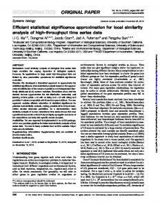
Fig. 1
Examples of IPPs locations.
of insufficient both temporal and spatial resolutions (Grejner-Brzezinska et al., 2004; Grejner-Brzezinska et al., 2006). Therefore, our research team has made an attempt to develop an accurate local ionosphere model for Polish territory that would support precise GNSS positioning and GNSS-based geodetic and geodynamic studies in the area of Poland (Bosy, 2005; Kontny and Bogusz, 2012). The main purpose of this initial study is to examine the accuracy of several TEC approximation techniques in providing the users grids with ionospheric delay corrections. Previous studies on the suitable approximation techniques for the ionosphere modeling include the Kriging and the Multiquadric Model (Wielgosz et al., 2003; Stanislawska et al., 1996; Stanislawska et al., 2002). This contribution, however, is an attempt to apply techniques that were used earlier in numerical terrain models (Declercq, 1996; Gosciewski, 2012). 2.
METHODOLOGY
For the ionospheric modeling, dual-frequency GPS data from Polish national ground based augmentation system (GBAS) - ASG-EUPOS - were used. This dense GPS network consisting of ~100 stations is a part of the European Position Determination System (EUPOS) project involving countries of Central and Eastern Europe (Bosy et al., 2008). In this study there was applied the methodology presented by Wielgosz et al. (2003), in which the ionospheric delay was computed using a geometry-free linear combination of carrier-phase smoothed pseudorange data. The differential code biases (DCB) for each station were estimated using methodology presented by (Komjathy et al., 2005), based on carrier-phase smoothed pseudorange data fitting into reference GIM. DCBs for GPS satellites were obtained from CODE AC. In order to represent the ionospheric TEC, a single layer model (SLM) ionosphere approximation was used (Schaer, 1999; Shagimuratov et al., 2002). This approach assumes that all free electrons are contained in a shell of infinitesimal thickness at
a fixed height. In the experiments presented here, the SLM height of 400 km was used. The vertical TEC (vTEC) at the ionospheric pierce points (IPP) was calculated by using a SLM mapping function (Lin, 2001). At the first step of the presented studies, analyses of IPP geometry for measurements of all ASG-EUPOS stations at each observational epoch were performed. For the TEC calculations an elevation mask of 20 degrees was used and the data processing with 30-second sampling interval was carried out. Figure 1 illustrates examples of IPP locations for the measurements collected at 00.00 UT and 20.20 UT on 9th March 2012. For every epoch, the observations from ~100 stations produce ~600 TEC measurements. White dots represent locations of the IPPs. As one can see, the IPP locations have a clustered distribution and are representative for other epochs over 24-hour period. As is shown, there are areas with a little or no data. This IPP distribution has crucial impact on the choice of the approximation techniques for ionospheric TEC interpolation and mapping. This suggests two approaches: a local and a general one. The local approach is based on a data fitting with two-dimensional functions with predefined search radius. This is performed for each grid point separately (one by one). The general approach is based on data fitting with twodimensional functions simultaneously for all IPPs at a particular epoch. It should be noted that the local approach produces non-continuous grids with TEC values provided for the locations around and within the IPP clusters. Nevertheless, this does not affect the usability of such grids in GNSS positioning, because the user located in the area of the reference network requires the ionospheric delay corrections only at IPPs within the clusters. The TEC values obtained from ASG-EUPOS GPS data at IPPs were interpolated using several approximation techniques in order to produce high-
VALIDATION OF APPROXIMATION TECHNIQUES FOR LOCAL TOTAL …
277
50
44o
45 40 35 30 25 20 15
10o
10 5 0 0
5
10
15
20
25
30
March 2012
Fig. 2
Variations of ∑Kp index during March 2012.
resolution instantaneous regional maps of the ionosphere. These presented and tested techniques are: NLP - near grid, local plane (search radius r = 6), NLP2 - near grid, local polynomial of second degree (search radius r = 3), NTL - near grid, local triangle weighting (search radius r = 6), LP - local plane (search radius r = 6), LP2 - local polynomial of second degree (search radius r = 3), TL - local triangle weighting (search radius. r = 6), GP2 - general polynomial of second degree, GP3 - general polynomial of third degree. The first six of the selected methods represent the local approach for ionospheric TEC mapping, these are: NLP, NLP2, NTL, LP, LP2, TL. As it was mentioned, the local techniques use separate approximation for each grid point. In addition, near grid methods generate grid points that are located within cluster areas only (Ehlschlaeger, 2002; Gosciewski, 2012). The general methods (GP2, GP3) provide a single (general) approximation for the whole area under consideration. 3.
NUMERICAL TESTS
The quality of the ionospheric maps was tested twofold. Firstly, by comparison to the high-quality CODE GIMs. Secondly, by creating DD ionospheric delay corrections and comparing them to highaccuracy reference values derived from the reference network data processing. All the approximation methods were analyzed for two different geomagnetic activity levels – on a disturbed day of March 9, 2012 (DOY 69) with ƩKp = 44o and max Kp reaching 8, and on a quiet day of March 20, 2012 (DOY 80) with ƩKp = 10o
(Fig. 2). This in turn allowed for testing the interpolation methods under various ionospheric activities. In this section, preliminary results of a comparative study of the most suitable interpolation techniques for local ionosphere mapping are presented. Figures 3 and 4 show ionospheric TEC maps provided by CODE AC (used as a reference) and selected three of eight tested interpolation methods: a near grid local plane approximation NLP, general polynomial of second degree GP2, local triangle weighting TL. The example maps are presented for both geomagnetic activity levels for afternoon hours. A computer program in Matlab language was created in order to perform required analyses. In the first step, TEC values at IPP were calculated for each data epoch. It should be noted that about 600 IPPs per epoch were computed. Next, local ionosphere maps were created with 5-minute interval using the tested approximation methods. The resulting spatial grid resolution was set to 0.25 x 0.25 degrees. The obtained grids cover the area spanning in latitude from 42⁰ N to 57⁰ N and in longitude from 3⁰ E to 38⁰ E. Figure 3 shows examples of the TEC maps at the selected epochs for the active ionosphere day. The comparison between the CODE maps and the maps derived with NLP and GP2 methods indicates rather good agreement. However, the CODE TEC level is slightly higher as compared to the maps generated using both methods. Also, the reference maps are smoother because of their global nature. On the other hand, it can be seen that the maps derived with the local triangle weighting method (TL) show small structures that are rather unrealistic. These features are mostly caused by the clustered distribution of IPPs and weak smoothing properties of TL method. Figure 4 presents examples of the TEC maps at the selected epochs for the quiet ionosphere day. Again,
278
A. Krypiak-Gregorczyk et al.
Fig. 3
Comparison between the ionosphere maps derived using NLP, GP2 and TL methods and CODE GIMs for the active day - 9 March 2012.
Fig. 4
Comparison between the ionosphere maps derived using NLP, GP2 and TL methods and CODE GIMs for the quiet day - 20 March 2012.
NLP and GP2 methods give a good agreement with CODE maps, and TL shows distinctive small structures. In addition, when comparing TEC values on the disturbed and quiet days, a negative phase of the ionospheric disturbances can be detected (Figs. 3 and 4).
AGREEMENT WITH CODE MAPS
The derived maps were compared to the CODE reference maps in order to study the accuracy of their absolute TEC level. In order to quantify the agreement of the tested ionosphere maps with the CODE GIMs, a relevant comparative study was carried out. It should be noted that the CODE maps are available
VALIDATION OF APPROXIMATION TECHNIQUES FOR LOCAL TOTAL …
279
Table 1 Statistics of the comparison of the ionospheric grids derived with the analyzed methods with CODE maps for the active and quite days. INTERPOLATION METHODS
09.03.2012 RMS
NLP NLP2 NTL LP LP2 TL GP2 GP3
Fig. 5
0.87 0.86 0.86 1.34 1.41 0.88 2.03 69.69
20.03.2012 mean -0.31 -0.25 -0.25 -0.55 -0.36 -0.28 -0.38 1.93
RMS 0.58 0.64 0.62 0.82 1.06 0.61 2.06 16.11
mean -0.31 -0.30 -0.30 -0.25 -0.31 -0.30 0.29 0.56
Differences between GP3- and GP2-derived maps and CODE GIM at 5:00 UT on 9 March 2012.
with 2-hour temporal resolution, hence, they needed to be interpolated in time to match tested 5-minute maps. TEC residuals between the grids derived from the tested interpolation techniques and the CODE maps were calculated and analyzed. Residual mean and root mean square error based on these residuals (calculated at each grid point over 24-hour period) are provided in Table 1. For all techniques, except GP3, the mean bias does not exceed 0.6 TECU (Fig. 5). In case of local interpolation approach, RMS errors do not exceed 1.5 TECU and, for most of the techniques, are lower than 1.0 TECU. Also, there is a clear storm effect; RMS errors are higher on the disturbed day in comparison to the quiet one. The best agreement is observed for NLP, NLP2, NTL and TL techniques. By contrast, the worst results were obtained with GP3 technique. This means that the 3rd order of the polynomial is too high and leads to unrealistic results. Another reason for poor performance of GP3 technique is the geometry of the IPPs (Fig. 5). The differences of over 20 TECU are observed in the areas without IPP coverage. In case of the areas with IPPs the residuals are much lower. In general, the local approaches present a good agreement with the CODE
product, and the obtained residuals lie within the limits of the official accuracy of the CODE maps. ACCURACY ANALYSIS OF DD IONOSPHERIC CORRECTIONS
The statistical analysis presented above showed the agreement of the local ionosphere maps with the CODE GIMs. However, further analysis are required in order to verify the applicability of the proposed ionosphere modeling techniques to precise positioning. In order to analyze the practical accuracy of the TEC maps (grids) generated with the tested approximation methods, the obtained TEC grids were used to calculate DD ionospheric delays of GNSS signals for two test baselines. Next, the model-derived DD delays were compared to the “true” reference DD ionospheric delays calculated for these two baselines over two 24-hour periods. The reference DD ionospheric delay values were obtained from solving a geometry-free linear combination of the carrierphase signals with introduction of the resolved integer ambiguities (Schaer, 1999; Grejner-Brzezinska et al., 2004).
A. Krypiak-Gregorczyk et al.
280
Fig. 6
Test baseline locations.
It should be noted that in the operational positioning scenario, these model-derived delays (denoted as “corrections” hereafter) are used for correction of GNSS observations in the high-precision positioning algorithms. The processing of static GNSS data collected during long sessions (e.g., several hours) does not require very accurate ionospheric information as a change in the satellite geometry allows for resolving the integer ambiguities. However, when processing short static sessions or kinematic data, the quality of the ionospheric information is crucial to the success of the ambiguity resolution process (Odijk, 2000; Wielgosz et al., 2005). This shows the importance of the correct ionospheric information in the precise positioning. In the faststatic or kinematic applications the expected accuracy of DD ionospheric corrections should be better than 10-20 cm. Table 2 Accuracy of DD ionospheric corrections for the active day - 9 March 2012. % of the residuals within the selected limits Baseline and model