Validity of Fresnel and Fraunhofer approximations in scalar diffraction

INSTITUTE OF PHYSICS PUBLISHING

JOURNAL OF OPTICS A: PURE AND APPLIED OPTICS

J. Opt. A: Pure Appl. Opt. 5 (2003) S86–S91

PII: S1464-4258(03)57211-7

Validity of Fresnel and Fraunhofer approximations in scalar diffraction Samir Mezouari and Andy Robert Harvey Electrical, Electronic and Computer Engineering, School of Engineering and Physical Sciences, Heriot-Watt University, Riccarton, Edinburgh EH14 4AS, UK

Received 2 December 2002, in final form 27 March 2003 Published 25 June 2003 Online at stacks.iop.org/JOptA/5/S86 Abstract Evaluation of the electromagnetic fields diffracted from plane apertures are, in the general case, highly problematic. Fortunately the exploitation of the Fresnel and more restricted Fraunhofer approximations can greatly simplify evaluation. In particular, the use of the fast Fourier transform algorithm when the Fraunhofer approximation is valid greatly increases the speed of computation. However, for specific applications it is often unclear which approximation is appropriate and the degree of accuracy that will be obtained. We build here on earlier work (Shimoji M 1995 Proc. 27th Southeastern Symp. on System Theory (Starkville, MS, March 1995) (Los Alamitos, CA: IEEE Computer Society Press) pp 520–4) that showed that for diffraction from a circular aperture and for a specific phase error, there is a specific curved boundary surface between the Fresnel and Fraunhofer regions. We derive the location of the boundary surface and the magnitude of the errors in field amplitude that can be expected as a result of applying the Fresnel and Fraunhofer approximations. These expressions are exact for a circular aperture and are extended to give the minimum limit on the domain of validity of the Fresnel approximation for plane arbitrary apertures. Keywords: Fresnel diffraction, Fraunhofer diffraction, near-field diffraction, far-field diffraction, scalar diffraction

(Some figures in this article are in colour only in the electronic version)

1. Introduction In scalar diffraction problems, evaluation of diffracted electromagnetic fields is often accomplished using either the Fresnel of Fraunhofer approximations. This demarcation is due to useful approximations, which greatly alleviate the complexity of evaluating the diffraction integrals. The general theory of diffraction at plane apertures was developed long ago [1–3] and is summarized in textbooks [4, 5]. The Fraunhofer approximation for diffraction from a planar aperture is in fact the Fourier transform of the aperture field distribution for which many highly optimized algorithms for the computation of Fourier transforms have been developed [6, 7]. In contrast, the Fresnel diffraction always involves the integration of a highly oscillatory function in the domain defined by the aperture, which makes its evaluation more difficult, although many approaches for dealing with this problem have been developed [8–10]. We build here on 1464-4258/03/040086+06$30.00 © 2003 IOP Publishing Ltd

earlier work by Shimoji [11] that showed that for diffraction from a circular aperture and for a specific phase error, there is a specific curved boundary surface between the Fresnel and Fraunhofer regions. The boundary between the Fraunhofer and Fresnel domains is determined by the relative size of the diffracting aperture and the displacement of the observation point as represented by the Fresnel number. Because of these mathematical approximations the location of the exact boundary is problematic. Southwell [12] studied, by direct numerical integration, the validity of the Fresnel approximation in the near field and found that it begins to break down for beams expanding faster than about f/12. Theoretical and experimental investigations of the Fresnel and Fraunhofer diffraction of a coherent light beam due to an elliptical aperture have been carried out and close agreement between them has been obtained [13]. The region where the Fresnel
approximation is valid is commonly given by z 3 > 25(a + x 2 + y 2 )4 /λ [5] where, as

Printed in the UK

S86

Validity of Fresnel and Fraunhofer approximations in scalar diffraction

V Y

(x, y, z)

X U

r

τ

(u, v, 0)

Z

σ

Aperture

Screen

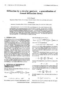
Figure 1. Diffraction of a plane wave from an arbitrary-shape planar aperture. r is the distance from point (u, v, 0) on the aperture to point (x, y, z) on the observation screen. σ is the distance between the aperture and the screen (normalized to wavelength). τ is the transverse distance between the Huygens source point (u, v, 0) and the observation point (x, y, z).

shown in figure 1, x, y, z are the Cartesian coordinates, a is the radius of the aperture and λ is the wavelength. This is obtained from the requirement for a specific maximum phase error. Steane and Rutt [14] explored the limits where the Fresnel approximation is valid by considering the propagation of waves in spatial-frequency space, and expressed the inaccuracy of the Fresnel approximation as directly related to the Fresnel number of the aperture. We derive here expressions for the regions of validity of both the Fresnel and Fraunhofer regions using the analytical expression of the Rayleigh–Sommerfeld integral, in the normal case of a circular aperture. In section 2 we use the scalar Kirchhoff diffraction formula to obtain an analytic expression for the optical field along the symmetric axis for a circular aperture. This enables comparison between Fresnel and Fraunhofer approximations along this axis. In section 3 we deduce the Fresnel and Fraunhofer regions from a simple phase error criterion combined with the error in amplitude and phase for the symmetric axis of circular aperture.

2. Background In scalar diffraction, the Kirchhoff formula with the first and second Rayleigh–Sommerfeld formulae, which describe the Huygens–Fresnel principle, are often used to represent the propagation of optical fields. Although the Rayleigh– Sommerfeld formulae and Kirchhoff diffraction are similar, further investigation shows that the Kirchhoff diffraction formula is a mathematically inconsistent theory [15–17]. The first Rayleigh–Sommerfeld formula gives a physically realistic prediction for the axial intensity close to a circular aperture, whereas the second Rayleigh–Sommerfeld and Kirchhoff diffraction formulae do not [18]. In this paper we are interested only in evaluating the surfaces that delineate the volumes for which the Fresnel and Fraunhofer diffraction theories are valid and these are not close to the diffracting aperture. It is therefore valid to use, as a starting position, any one of the three above diffraction formulae. We have chosen to use the second Rayleigh–Sommerfeld formula since it is both accurate in this space range and, importantly, can be readily solved analytically.

To study the validity of the Fresnel approximation, the propagation of the optical wave front A(u, v, 0) from the plane containing the aperture therefore requires only the evaluation of the second Rayleigh–Sommerfeld formula (for plane waves) and is defined as    1 ∂ A(u, v, z)  eikr E(x, y, z) = − du dv, (1)  2π ∂z  z=0 r where  determines the boundaries of integration, r =
z 2 + (x − u)2 + (y − v)2 and k = 2π . λ The area of integration over the aperture requires, in general, two-dimensional manipulations. However, when the aperture function is separable in a specific coordinate system, the problem is reduced to one-dimensional manipulation [15]. For circular apertures the use of polar coordinates, u = ρ cos θ and v = ρ sin θ , allows the separation of components and equation (1) can be written as √   2 2 i 2π a eik z +ρ
ρ dρ dθ. (2) E(0, 0, z) = − λ 0 z2 + ρ2 0 Consider a circular aperture
irradiated by a plane wave with unity amplitude and let R = z 2 + ρ 2 be the distance between a given Huygens source and the observation point, so that equation (2) is reduced to a one-dimensional integral:  √z 2 +a 2 i 2π eik R dR E(0, 0, z) = − λ z = eikz − eik

√

z 2 +a 2

.

(3)

Equation (3) gives the analytical expression of the field amplitude along the symmetric z-axis behind a circular aperture illuminated by plane waves with unity amplitude. Its form is shown in figure 2 for a/λ = 1000. It should be noticed that the second Rayleigh–Sommerfeld diffraction formula is valid only when the dimensions of the aperture and the distance from the aperture to the observation point are large compared to the wavelength. As emphasized above, the direct calculation of equation (1) is an intractable problem; however, in certain cases such as along the symmetric axis as, in the evaluations here, it is possible to derive analytical solutions [19]. S87

S Mezouari and A R Harvey

3. Fresnel and Fraunhofer regions In this section we derive the domains in which the Fresnel and Fraunhofer approximations are valid. In order to simplify the mathematics we employ normalized coordinates (x − u)2 + (y − v)2 , λ2

τ2 =

(10)

z , (11) λ where τ is the normalized lateral displacement between the source of the secondary wavelet at (u, v) and the observation point at (x, y). Writing the phase in the integrand in equation (4) as the Maclaurin series (equation (5)) in terms of τ and σ yields σ =

Figure 2. The amplitude |E(0, 0, z)| along the symmetric z-axis for a circular aperture with radius a/λ = 1000. The spatial coordinates are expressed in terms of wavelength λ.

To simplify evaluation of the Fresnel–Kirchhoff integral, the general assumption states that variations in the argument of the exponent have a greater effect than variation in other terms. Thus, equation (1) becomes   i A(u, v, 0)eikr du dv. (4) E(x, y, z) = − λz 

 3   τ 1 τ2 +O , = 2π σ + 2σ σ

where the higher-order terms O( στ )3 are neglected in the Fresnel approximation. These terms correspond to the phase error due to the Fresnel approximation. The maximum error introduced by the truncation of the MacLaurin series in the Fresnel approximation is

To simplify the argument of the exponent, the r -term can be replaced by the Maclaurin series expansion (x − u)2 + (y − v)2 ((x − u)2 + (y − v)2 )2 + ··· r =z+ + 2z 8z 3 (5) and to apply the Fresnel approximation only the first two terms in this expansion are retained. We thus obtain r ≈z+

(x − u)2 + (y − v)2 . 2z

Equation (4) is then rewritten to yield the Fresnel near-field, diffraction integral:   (x−u)2 +(y−v)2 i 2z A(u, v, 0)eik du dv. E(x, y, z) = − eikz λz  (7) When r is large, the aperture dimension can be neglected compared to the distance z (z  u, v), which can be applied to expression (6) to yield r =z+

x 2 + y 2 − 2xu − 2yv + ···. 2z

(8)

Substitution of (8) into (7) gives the Fraunhofer approximation:   x 2 +y 2 xu+yv i A(u, v, 0)e−ik z du dv. E(x, y, z) = − eikz eik 2z λz  (9) Although these two approximations to the exact scalar diffraction integral are conceptually similar, the numerical and analytical evaluation of the Fresnel approximation is generally more challenging. Fortunately, the Fraunhofer diffraction is the most important case encountered in engineering optics. Notice, in (9), that Fraunhofer diffraction by an aperture is the Fourier transform of the aperture field distribution. S88

fh = −

π τ4 . 4 σ3

(13)

If we choose a maximum allowable error max,Fres that we can tolerate by employing the Fresnel approximation, then this determines the domain for which the Fresnel approximation introduces this error to be the domain defined by 

(6)

(12)

τ