Fresnel diffraction and fractal patterns from polygonal ... - CiteSeerX

2768

J. Opt. Soc. Am. A / Vol. 23, No. 11 / November 2006

Huang et al.

Fresnel diffraction and fractal patterns from polygonal apertures J. G. Huang, J. M. Christian, and G. S. McDonald Joule Physics Laboratory, Institute for Materials Research, School of Computing, Science and Engineering, University of Salford, Salford M5 4WT, UK Received April 28, 2006; accepted June 7, 2006; posted June 20, 2006 (Doc. ID 70311) Two compact analytical descriptions of Fresnel diffraction patterns from polygonal apertures under uniform illumination are detailed. In particular, a simple expression for the diffracted field from constituent edges is derived. These results have fundamental importance as well as specific applications, and they promise new physical insights into diffraction-related phenomena. The usefulness of the formulations is illuminated in the context of a virtual source theory that accounts for two transverse dimensions. This application permits calculation of fractal unstable-resonator modes of arbitrary order and unprecedented accuracy. © 2006 Optical Society of America OCIS codes: 050.1220, 050.1960, 140.3410, 260.1960, 140.0140.

1. INTRODUCTION In scalar diffraction theory, the semi-infinite space beyond an aperture contains two paraxial regions—the near field and the far field—where Fresnel and Fraunhofer theories are valid, respectively. While analytical descriptions of Fraunhofer patterns from regular-polygon apertures have been known for many years,1–3 there appears to be almost no published material on the corresponding Fresnel patterns. The lack of development in this area is reflected in standard textbooks,4–7 where near-field treatments tend to be restricted to considerations of infinite straight edges and of closed apertures with rectangular and circular shapes. In each of these cases, the Fresnel patterns are essentially one-dimensional in character. In this paper, we present two complementary analytical techniques for calculating the Fresnel diffraction patterns from hard-edged polygonal apertures illuminated by a plane wave. These frameworks are exact, in that they do not involve any further approximation beyond the (paraxial) Fresnel diffraction integral. We consider regular polygonal apertures, but the approaches can be readily extended to describe near-field diffraction from closed apertures of arbitrary shape. Our results are of fundamental importance and have specific applications where standard methods, such as fast Fourier transform (FFT) techniques, fail. For example, in unstableresonator-mode calculations, both (paraxial beam) ABCD matrix modeling and existing semi-analytical methods can give accurate results only in limited parameter regimes in which the Fresnel number of the resonator is low. Consequently, a complete and detailed study of the fractal laser modes arising from unstable cavities8–13 has not previously been possible. A specific advantage of our formalisms over, for example, FFT-based methods is their ability to calculate the fine details of only a small portion of one, or many, complex diffraction patterns. It is this property that allows us to apply our results in the calculation of fractal laser modes of unprecedented accuracy. 1084-7529/06/112768-7/$15.00

The explicit mathematical form of our results may also lend physical insight into other diffraction-related phenomena in physics; for example, the origins of excess quantum noise in lasers, where the transverse symmetry of the aperturing element has been shown to play a central role in the observed phenomena.14–17 In Fraunhofer theory, the far-field approximation allows diffraction patterns and derivative concepts (for example, holography, filtering, convolution, and coherence) to be expressed in terms of simple Fourier integrals and transform theorems, respectively. Our main results describe the physical and mathematical character of near-field diffraction patterns in terms of their elemental spatial structures (edge waves). It is also plausible that our results could open future doors in the development of derivative concepts in Fresnel optics.

2. THEORY When a plane monochromatic wave of complex amplitude U0 illuminates a hard-edged aperture, the field U共x , y兲 in a plane at distance L beyond the aperture can be expressed as the area integral4,5

U共x,y兲 =

kU0 2␲iL

冕冕

再

d␰d␩ exp i

⍀

k 2L

冎

关共x − ␰兲2 + 共y − ␩兲2兴 , 共1兲

where k is the wavenumber of the incident plane wave and ⍀ denotes the aperture area (see Fig. 1). 共x , y兲 and 共␰ , ␩兲 are the observation- and aperture-plane coordinate axes, respectively. The paraxial approximation, employed in the derivation of the Fresnel diffraction integral (1), strictly requires the inequality L3
kb4 / 8 to be satisfied, where b is the largest characteristic length associated with the aperture. © 2006 Optical Society of America

Huang et al.

Vol. 23, No. 11 / November 2006 / J. Opt. Soc. Am. A

c共␹j兲 =

s共␹j兲 =

Fig. 1. Schematic diagram illustrating the coordinate system used to describe diffraction patterns from an aperture ⍀ illuminated by a plane wave of amplitude U0.

Within an edge-wave representation of diffraction patterns, the field in the observation plane is regarded as the superposition of the transmitted plane wave and an edgewave field E共x , y兲 arising from the boundary of the aperture:4 U共x,y兲 = ␧U0 + E共x,y兲.

共2兲

Here, ␧ is equal to unity if the point 共x , y兲, lies within the bright geometrical shadow of the aperture, and is zero if it is outside this region. We now express the edge-wave field in terms of two different formulations to obtain two methods for calculating the resulting Fresnel diffraction patterns. Results are then presented and a brief comparison of the two methods is made. A. S-Function Method Our first approach is based upon exploiting the mathematical framework introduced by Silverman and Strange.18 We define the dimensionless relative spatial coordinates u = 冑2 / ␭L共x − ␰兲 and v = 冑2 / ␭L共y − ␩兲 that simplify the Fresnel diffraction integral (1) to U共x,y兲 =

U0 共1 + i兲2

冕冕 ⍀

冋

␲

册

dudv exp i 共u + v 兲 . 2 2

2

S共␹1, ␹2兲 = − 1 +

共1 + i兲

冕

冉 冊

␹2

␲

dv exp i v2 . 2

where D共␹j兲 = −

冉 冊

␲ ␾*共␹j兲exp i ␹j2 , 1+i 2 i

1

− f共␹j兲cos

2

2

␲ 2

冉 冊 冉 冊 ␲

␹j2 − g共␹j兲cos

2

␲

␹j2 − g共␹j兲sin

1 + 0.926␹j

f共␹j兲 =

g共␹j兲 =

2

␹j2 ,

共7a兲

␹j2 ,

共7b兲

2 + 1.792␹j + 3.104␹j2

共8a兲

,

1 2 + 4.142␹j + 3.492␹j2 + 6.67␹j3

共8b兲

.

When ␹j ⬍ 0, the auxiliary functions are evaluated using

冋

冉 冊 ␲

f共− 兩␹j兩兲 = f共兩␹j兩兲 − 2 c共兩␹j兩兲sin

2

冉 冊册 ␲

␹j2 − s共兩␹j兩兲cos

2

␹j2

,

共9a兲

冋

冉 冊

g共− 兩␹j兩兲 = g共兩␹j兩兲 + 2 c共兩␹j兩兲cos

␲ 2

冉 冊册

␹j2 + s共兩␹j兩兲sin

␲ 2

␹j2

,

共9b兲 These relations follow from consideration of the symmetry of the Fresnel integrals. By substituting Eq. (4) into Eq. (3), one obtains

冋

共3兲

1

共4兲

The ␹j共j = 1 , 2兲 limits denote the boundary of an infinite slit aperture in one direction. Physically, S represents the edge-wave pattern from this slit when the slit is illuminated by a unit plane wave, and this can be written as a superposition of two components (from the constituent edges): S共␹1, ␹2兲 = D共␹1兲 + D共− ␹2兲,

2

␲

U共x,y兲 = U0 1 + S共u2,u1兲

To facilitate the analytical evaluation of the area integral (3), we introduce the following S-function: ␹1

+ f共␹j兲sin

where c共␹j兲 = 兰0␹j cos共␲␶2 / 2兲d␶ and s共␹j兲 = 兰0␹j sin共␲␶2 / 2兲d␶ are the familiar Fresnel cosine and sine integrals, respectively. The auxiliary Fresnel functions can be evaluated efficiently using rational approximations of the required accuracy.19 When ␹j is nonnegative, one may choose

+

1

冉 冊 冉 冊

1

2769

1+i

冕

u2

u1

冉 冊册

␲ duS关v1共u兲,v2共u兲兴exp i u2 2

, 共10兲

where v1共u兲 and v2共u兲 are parametric expressions describing the shape of the aperture in the relative coordinate system (see Fig. 2). The edge-wave field E共x , y兲 is then given by Eq. (2). In many cases it proves to be more efficient to consider a specific aperture shape as broken down into an assembly of subapertures. Babinet’s principle can then be employed to generate diffraction patterns. Here we focus our attention on apertures that are regular polygons. For a polygon with N sides, the most obvious decom-

共5兲

共6a兲

and

␾共␹j兲 ⬅ f共␹j兲 + ig共␹j兲.

共6b兲

The auxiliary Fresnel functions, f and g, and defined through

Fig. 2. Schematic diagram of an aperture of arbitrary shape in the relative coordinates 共u , v兲.

2770

J. Opt. Soc. Am. A / Vol. 23, No. 11 / November 2006

Huang et al.

B. Line-Integral Method In this formulation, we define two vectors in complexnumber notation, p = x + iy and q = ␰ + i␩, and recast the Fresnel diffraction integral (1) as

U共p兲 = Fig. 3. Two schemes for dividing a regular polygon into subapertures: (a) a triangle ensemble, and (b) a combination of other shapes.

position is that involving N congruent isosceles triangles [Fig. 3(a)], each of which has a diffraction pattern that can be calculated with Eq. (10). Babinet’s principle can then be stated as U共x,y兲 = U0␧ + E共x,y兲,

共11a兲

kU0 2␲iL

冕冕

冉

d2q exp i

⍀

k 2L

冊

兩p − q兩2 .

共13兲

By applying a low-dimensional divergence theorem, Eq. (13) can be transformed from an integral over the planar area of the aperture to one around its simple closed-curve boundary.20,21 The diffraction integral (13) is then given by the circulation,

冋

U共p兲 = U0 ␧ −

1 2␲

冖 冉

k

exp i

␴

2L

兩q − p兩2

冊

q−p 兩q − p兩2

册

· ndl , 共14兲

where N

E共x,y兲 ⬅

兺 E 共x,y兲,

共11b兲

j

j=1

For an isosceles triangle [e.g., triangle 1 in Fig. 3(a)] of half-angle ␪ = ␲ / N, whose vertex is at the origin and whose perpendicular length a is aligned along the ␰-axis, the edge-wave contributions are given by

冋

E共x⬘,y⬘兲 = U0 关1 − ␧ + S共x⬘,x⬘ − A兲兴

冕

x⬘

冉 冊册

␲ duS共w1,w2兲exp i u2 1 + i x⬘−A 2 1

+

, 共12a兲

where n is the unit outward normal vector to the edge (within the aperture plane), dl is the line element along the edge, and ␴ denotes the aperture boundary. The parameter ␧ is equal to unity if point p lies within the bright geometric projection of this aperture, and it is zero if p is outside this region. For a polygonal aperture (see Fig. 4), the position of a vertex Aj is given by the position vector qj. It is also convenient to define vectors Lj = qj+1 − qj, tj = Lj / Lj, and nj (denoting the unit outward normal of side Lj). The position vector of a general point on the side of length Lj can then be represented as q = qj + tjl, where l is the distance from the vertex Aj. Using these constructs, it is possible to rewrite Eq. (14) in a form more suitable for describing the diffraction pattern from an N-sided regular polygon:

冋

where w1共u,x⬘,y⬘, ␪兲 = y⬘ − 共u − x⬘兲tan ␪ ,

共12b兲

w2共u,x⬘,y⬘, ␪兲 = y⬘ + 共u − x⬘兲tan ␪ ,

共12c兲

and A = a冑2 / ␭L. An intuitive way of generating the edgewave pattern of each of the other component triangles [e.g., triangles 2, 3 , . . ., and 8 in Fig. 3(a)] is through rotational transformation. A rotational transform of an angle ␾ in the aperture plane is equivalent to considering the system with new observation-plane coordinates x⬘ = x cos ␾ + y sin ␾ and y⬘ = y sin ␾ − x cos ␾. However, we find that a more efficient approach to the N-sided polygonal aperture problem is to replace triangle ensembles with combinations of triangles and trapezoids [see Fig. 3(b)]. In cases with an even number of sides, one can also exploit the presence of a central rectangle. For example, calculations for an octagonal aperture require just two integrations—one for each trapezoid on either side of this rectangle. In contrast, adding together eight triangles, each with half-angle ␪ = ␲ / 8 and with a diffractive contribution resembling Eq. (12), could require eight integrations (one per triangle). Triangle ensembles are therefore not necessarily efficient computational constructs, though the physical symmetry of the problem is more explicitly preserved when they are used.

U共p兲 = U0 ␧ −

1

N

兺 I 共q ,t 兲

2␲ j=1

j

j

j

册

,

共15兲

where

冕 冉 Lj

Ij共qj,tj兲 =

exp i

0

k 2L

兩qj + tjl − p兩2

冊

q j + t jl − p 兩qj + tjl − p兩2

• njdl. 共16a兲

After some manipulation, Eq. (16a) can be simplified to

Fig. 4. Geometrical constructs used in the formulation of the line-integral method.

Huang et al.

Vol. 23, No. 11 / November 2006 / J. Opt. Soc. Am. A

冉

Ij共qj,tj兲 = 共qj − p兲 · nj exp i ⫻

冕

k 2L

Lj+共qj−p兲·tj

共qj−p兲·tj

兩共qj − p兲 · nj兩2

冊 冉 冊 k

dl l + 兩共qj − p兲 · nj兩 2

2

2771

exp i

2L

l2 . 共16b兲

The edge-wave field, in the line-integral representation, is then expressed as E共p兲 =

U0

N

兺 I 共q ,t 兲.

2␲ j=1

j

j

j

共17兲

The physical meaning of Eq. (17) is obvious—the total edge wave from the aperture is a sum of the edge-wave contributions arising from each of the straight edges, of finite length, that make up the aperture. These individual contributions, each represented by a line integral, are of a more involved and general character than the relatively trivial, but more familiar, contributions that arise from straight edges of infinite length. Equation (15), combined with Eq. (16b), can be used to calculate Fresnel diffraction patterns from a polygonal aperture of nonregular shape and with an arbitrary number of sides. The formulation of the diffractive wave contribution from each straight edge of a closed aperture, Eq. (16), is a key result of this paper that invites geometrical interpretation. The relative transverse displacement and orientation of the observation point p and the jth edge of the aperture are found to be expressed in terms of new orthogonal coordinates that map perpendicular distance, 共qj − p兲 · nj, to the line of the edge and the displacement of apex Aj from p along a direction parallel to this edge, 共qj − p兲 · tj. For an N-sided regular polygonal aperture, one can set qj = R cos共␸0 + 2␲j/N兲 + iR sin共␸0 + 2␲j/N兲,

共18a兲

pm = r cos共␪0 + 2␲m/N兲 + ir sin共␪0 + 2␲m/N兲, 共18b兲 where ␸0 and ␪0 are arbitrary constants. Then, 共qj − pm兲 · nj = 共qj+1 − pm+1兲 · nj+1 ,

共19c兲

共qj − pm兲 · tj = 共qj+1 − pm+1兲 · tj+1 ,

共19d兲

and

Substitution of these results into Eq. (15) yields U共pm兲 = U共pm+1兲,

共20兲

demonstrating mathematically that the diffraction pattern of an N-sided regular polygonal aperture has N-fold rotational symmetry. Finally, we note that the integrand in Eq. (16b) oscillates more rapidly as L is decreased. As expected, an accurate computation of the integrals thus requires the number of sampling points to be increased as the observation plane approaches the aperture. C. Fresnel Diffraction Patterns The S-function and line-integral approaches have been used to calculate the diffraction patterns for N-sided regular-polygonal apertures with N = 3 to N = 10. The numerical integrations are calculated using an extended trapezoidal rule. When denoting x0 , x1 , . . . , xN as a se-

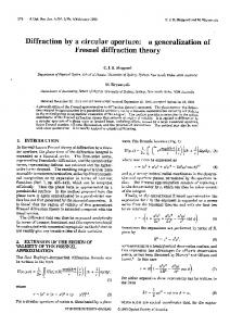
Fig. 5. (Color online) Fresnel patterns (normalized intensity distribution, defined by 兩U共x , y兲兩2 / U02) from (a) triangle, (b) pentagon, (c) hexagon, and (d) decahedron apertures.

quence of equally-spaced positions, separated by a constant step h (xi = x0 + ih and i = 1 , . . . , N), the integration of a function f共x兲 in the interval 关x0 , xN兴, 兰xxNf共x兲dx, is ap0 proximated as h 关f0 / 2 + f1 + ¯ + fN−1 + fN / 2兴, where fi ⬅ f共xi兲 is the value of the function at position xi. For brevity, we present only a selection of patterns: those for the isosceles triangle 共N = 3兲, the pentagon 共N = 5兲,the hexagon 共N = 6兲, and the decahedron 共N = 10兲. These are shown in Fig. 5. The optical wavelength was chosen to be ␭ = 0.5 ␮m, corresponding to illumination with green light that is readily obtainable from a green laser pointer. It is thus straightforward to reproduce these patterns experimentally. The radial distance R from the center of the polygon to a circle enclosing the aperture (upon whose circumference all apices lie) is taken as R = 1 mm, and the distance between aperture and image planes is set to L = 100 mm (satisfying the paraxiality condition). Figure 5 shows that the pattern acquires an increasing degree of fine structure as N increases. As predicted by Eq. (20), patterns from N-sided regular polygonal apertures have N-fold rotation symmetry. Also, corners with smaller angles tend to contribute more widely diffracted light. Figure 6 demonstrates typical variation in the Fresnel pattern as the observation plane moves toward the aperture plane. A definition of the Fresnel number Feff for polygons given in Ref. 22 a2 Feff =

␭L

1 +

f共N兲

,

共21兲

where, as earlier, a is the radius of the inscribed circle of the polygon. Equation (21) contains two terms; the first is the conventional Fresnel number for a circular aperture, and the second has been proposed to account for additional pattern detail arising from the geometrical nature of the aperture, where

2772

J. Opt. Soc. Am. A / Vol. 23, No. 11 / November 2006

f共N兲 = 0.30618N2 − 0.10533N − 0.68095.

Huang et al.

共22兲

For example, Feff can vary with either a change in the number of aperture sides (see Fig. 5) or a change in L for a fixed aperture (see Fig. 6). D. Comparison of Methods The diffraction patterns calculated using the S-function and line-integral approaches have been checked independently using the standard FFT method.23 The three methods have their own distinct advantages and disadvantages. For a single, complete, and low Feff pattern that is sampled with a uniform transverse grid, the FFT approach is most efficient. This is because the other methods can require many numerical integrations. For example, a decahedron aperture many involve four integrations using the S-function method (assuming appropriate aperture decomposition), while the line-integral method could involve one integration per polygon side. However, FFT methods involve computation of complete diffraction patterns and further require the use of spatial grids that sample a sufficient amount of the dark background surrounding each pattern. When one requires accurate knowledge of the detailed structure of one or many higher Feff patterns or sections of high resolution patterns (e.g., dense and/or nonuniform sampling of a small area), or simply calculation of the optical field at a single transverse point, then the efficiency of the other two methods tends to be far greater. Implementation of the FFT approach in such contexts can also lead to reduced accuracy in the data acquired. Deployment of rational approximations in the S-function method introduces some truncation errors, but highaccuracy approximations24,25 can be used without entailing great computational overhead. Finally, the numerical

accuracy of the line-integral approach, which can be the most time-consuming, is essentially limited only by machine precision. Our original motivation for the reformulations of the Fresnel diffraction problem was the complete failure of FFT approaches in two-dimensional (2D) transverse unstable-resonator mode calculations when moderate-tohigh cavity Fresnel numbers were considered.26 The resolution of this problem, which involves the superposition of sections from very many distinct diffraction patterns of widely varying size, is detailed in the following section.

3. EXAMPLE OF APPLICATION The virtual source (VS) method26–30 is a semi-analytical technique that unfolds an unstable cavity into a sequence of equivalent virtual apertures. Accurate approximations of the cavity mode profiles can be obtained using a weighted summation of edge waves diffracted from these apertures. In particular, computation of 2D unstablecavity eigenmodes using this approach requires knowledge of only sections of the patterns from these aperturing elements. Moreover, the sampling density of the final mode pattern dictates the resolution of each of these pattern sections. FFT methods can be used for calculating edge-wave patterns (as an alternative to Fresnel integral approximations). This works well in one-dimensional VS codes. However, the FFT approach becomes impractical when fully 2D virtual apertures are involved (due to the demands placed on computer memory and processing time). A distinct advantage over existing (fully numerical) Fox–Li techniques31 for calculating unstable-cavity laser modes is that virtual source approaches enable the simultaneous calculation of a whole family of modes. In contrast, the Fox–Li algorithm needs to be manipulated nontrivially when dealing with different higher-order modes, and in each application only a single pattern can be obtained.30 We consider a geometrically unstable resonator with a single polygonal aperturing element whose edge is represented by the equation h共␰ , ␩兲 = 0. After the cavity is unfolded, the edge of the kth virtual aperture of the system can be described by the equation hk ⬅ h共␰M−k, ␩M−k兲 = 0,

共23兲

where M is the magnification of the resonator. This virtual source of diffracted waves is located at a longitudinal position Zk relative to the center of the aperture, where M2k − 1 Zk = BM

M2 − 1

共24兲

,

and B is the second element of its ABCD matrix.23 The mode profile V共x , y兲 of the unstable resonator is then represented by the weighted superposition27–30 V共x,y兲 = e0 Fig. 6. (Color online) Fresnel patterns from a triangular aperture with different Fresnel number Feff. (a) Feff = 3.06, L = 200 mm; (b) Feff = 3.89, L = 150 mm; (c) Feff = 7.23, L = 75 mm; (d) Feff = 10.56, L = 50 mm. (In each case, R = 1 mm and ␭ = 0.5 ␮m).

冋

ENs+1共xc,yc兲

␣Ns共␣ − 1兲

Ns

+

兺␣

k=1

−k

册

Ek共x,y兲 ,

共25兲

where Ns is the number of virtual sources and Ek共x , y兲 is the edge wave generated at the kth aperture; Ek共x , y兲 can be calculated by using either the S-function or line-

Huang et al.

Vol. 23, No. 11 / November 2006 / J. Opt. Soc. Am. A

integral method, and 共xc , yc兲 represents the coordinates of an arbitrary point on the boundary of the system aperture. For polygonal apertures, we choose this to be the point farthest from the center of the aperture. e0 is the planar field amplitude at the point 共xc , yc兲 in the output plane. In Eq. (25), ␣ is the mode eigenvalue satisfying the polynomial equation27–29 Ns

␣Ns+1 +

兺 关E 共x ,y 兲 − E k

c

c

k+1共xc,yc兲兴␣

Ns−k

= 0,

共26兲

k=0

where E0共xc , yc兲 = −1. The accuracy of the 2DVS calculation increases as Ns → ⬁. Southwell suggested that to ensure a reliable result, the number of virtual sources must be chosen so that Ns ⬎ log共250Neq兲 / log共M兲, where the equivalent Fresnel number Neq of an unstable resonator is given by23 Neq =

冉 冊冉 冊 a2

M2 − 1

␭B

2M

共27兲

and ␭ is the wavelength of the intracavity field. An alternative expression for the required number of virtual ap-

2773

ertures is given in Ref. 30. To demonstrate our 2DVS method, first we calculate the lowest order mode of an unstable resonator with the same (low Fresnel number) parameters used by Berry [see Fig. 4(a) of Ref. 32]. Our result, shown in Fig. 7, is completely consistent with Berry’s asymptotic prediction that employs trigonometric approximations of the Fresnel integrals. Second, we apply our method to calculate the lowest-order modes of resonators with higher Fresnel numbers and with triangular, pentagonal, hexagonal, and decahedral apertures. These results are shown in the upper row of Fig. 8. The lower row of panels in Fig. 8 shows a magnification of the central region of each pattern. For each configuration, the generic fractal signature of a high degree of fine structure within larger scale structure is clearly evident. To the best of our knowledge, these fractal eigenmodes are the most detailed and accurate patterns that have so far been obtained from theoretical calculation. Opportunities are thus opened up for detailed comparisons with more recent experiment results33 and for modeling novel applications of such fractal light.

4. CONCLUSIONS

Fig. 7. (Color online) Lowest-order mode of an unstable resonator with triangular aperture (M = 4, Neq = 7.4604, R = 1 mm).

We have presented two complementary analytical descriptions of Fresnel diffraction patterns from polygonal apertures. Two different, but entirely equivalent, mathematical routes have been taken to formulate this problem, and supporting numerical work has verified that they produce identical results. The two analytical forms for the edge waves concerned provide a potential physical framework for interpreting diffraction-related phenomena in the Fresnel regime. They also make possible an accurate generalization of Southwell’s virtual source method to include two transverse dimensions.26,32 This can allow calculation of 2D eigenmode patterns with arbitrary order and to unprecedented accuracy. Further applications may, for example, be possible in the area of understanding excess quantum noise,34,35 where the transverse symmetry of a resonator is known to have a significant effect.14–16

Fig. 8. (Color online) Lowest-order modes of unstable resonators (M = 1.5, R = 1 mm) with (a) triangular 共Neq = 12.5兲, (b) pentagonal 共Neq = 32.725兲, (c) hexagonal 共Neq = 37.5兲, and (d) decahedral 共Neq = 45.225兲 apertures. Note that a redefinition of a to be the radius of the circumcircle of each polygon yields a value of 50 for Neq in each of these four configurations.

2774

J. Opt. Soc. Am. A / Vol. 23, No. 11 / November 2006

ACKNOWLEDGMENTS This work is supported by Overseas Research Studentship award 2002035004 and the University of Salford.

REFERENCES 1. 2. 3.

4. 5. 6. 7. 8. 9. 10. 11. 12. 13. 14. 15. 16.

R. C. Smith and J. S. Marsh, “Diffraction patterns of simple apertures,” J. Opt. Soc. Am. 64, 798–803 (1974). J. Komrska, “Simple derivation of formulas for Fraunhofer diffraction at polygonal apertures,” J. Opt. Soc. Am. 72, 1382–l384 (1982). S. Ganci, “Simple derivation of formulas for Fraunhofer diffraction at polygonal apertures from Maggi—Rubinowicz transformation,” J. Opt. Soc. Am. A 1, 559–561 (1984). M. Born and E. Wolf, Principles of Optics, 6th ed. (Pergamon, 1980). E. Hecht, Optics, 4th ed. (Addison Wesley, 2002). G. Brooker, Modern Classical Optics (Oxford University, 2003). F. A. Jenkins and H. E. White, Fundamentals of Optics, 4th ed. (McGraw-Hill, 1981). G. P. Karman and J. P. Woerdman, “Fractal structure of eigenmodes of unstable cavity lasers,” Opt. Lett. 23, 1909–1911 (1998). G. P. Karman, G. S. McDonald, G. H. C. New, and J. P. Woerdman, “Laser optics—fractal modes in unstable resonators,” Nature 402, 138 (1999). G. S. McDonald, G. P. Karman, G. H. C. New, and J. P. Woerdman, “Kaleidoscope laser,” J. Opt. Soc. Am. B 17, 524–529 (2000). G. H. C. New, M. A. Yates, J. P. Woerdman, and G. S. McDonald, “Diffractive origin of fractal resonator modes,” Opt. Commun. 193, 261–266 (2001). M. A. Yates and G. H. C. New, “Fractal dimension of unstable resonator modes,” Opt. Commun. 208, 377–380 (2002). C. M. G. Watterson, M. J. Padgett, and J. Courtial, “Classic-fractal eigenmodes of unstable canonical resonators,” Opt. Commun. 223, 17–23 (2003). G. P. Karman, G. S. McDonald, J. P. Woerdman, and G. H. C. New, “Excess-noise dependence on intracavity aperture shape,” Appl. Opt. 38, 6874–6878 (1999). G. S. McDonald, G. H. C. New, and J. P. Woerdman, “Excess noise in low Fresnel number unstable resonators,” Opt. Commun. 164, 285–295 (1999). M. A. van Eijkelenborg, Å. M. Lindberg, M. S. Thijssen, and J. P. Woerdman, “Influence of transverse resonator symmetry on excess noise,” Opt. Commun. 137, 303–307 (1997).

Huang et al. 17. 18. 19. 20. 21. 22. 23. 24. 25. 26.

27. 28. 29. 30. 31. 32. 33.

34.

35.

M. V. Berry, “Mode degeneracies and the Petermann excess-noise factor for unstable lasers,” J. Mod. Opt. 50, 63–81 (2003). M. P. Silverman and W. Strange, “The Newton two-knife experiment: Intricacies of wedge diffraction,” Am. J. Phys. 64, 773–787 (1996). M. Abramowitz and I. A. Stegun, Handbook of Mathematical Functions (Wiley-Interscience, l972). J. H. Hannay, “Fresnel diffraction as an aperture edge integral,” J. Mod. Opt. 47, 121–124 (2000). J. S. Asvestas, “Line integrals and physical optics. Part II. The conversion of the Kirchhoff surface integral to a line integral,” J. Opt. Soc. Am. A 2, 896–902 (1985). S. M. Wang, Q. Lin, L. P. Yu, and X. L. Xu, “Fresnel number of a regular polygon and slit,” Appl. Opt. 39, 3453–3455 (2000). A. E. Siegman, Lasers (University Science Books, 1986). K. D. Mielenz, “Computation of Fresnel integrals,” J. Res. Natl. Inst. Stand. Technol. 102, 363–365 (1997). K. D. Mielenz, “Computation of Fresnel integrals. II,” J. Res. Natl. Inst. Stand. Technol. 105, 589–590 (2000). G. S. McDonald, G. H. C. New, and J. P. Woerdman, “The two-dimensional virtual source method,” presented at the 14th National Quantum Electronics Conference, Manchester, UK, September 6–9, 1999. W. H. Southwell, “Virtual-source theory of unstable resonator modes,” Opt. Lett. 6, 487–489 (1981). W. H. Southwell, “Unstable-resonator-mode derivation using virtual-source theory,” J. Opt. Soc. Am. A 3, 1885–1891 (1986). M. Berry, C. Storm, and W. van Saarloos, “Theory of unstable laser modes: edge waves and fractality,” Opt. Commun. 197, 393–402 (2001). M. A. Yates, G. H. C. New, and T. Albaho, “Calculating higher-order modes of one-dimensional unstable laser resonators,” J. Mod. Opt. 51, 657–667 (2004). A. G. Fox and T. Li, “Resonator modes in a maser interferometer,” Bell Syst. Tech. J. 40, 453–488 (1961). M. V. Berry, “Fractal modes of unstable lasers with polygonal and circular mirrors,” Opt. Commun. 200, 321–330 (2001). J. A. Loaiza, E. R. Eliel, and J. P. Woerdman, “Experimental observation of fractal modes in unstable optical resonators,” arXiv:physics/0304046 vl, 11 Apr, 2003, (http://arxiv.org/PS_cache/physics/pdf/0304/0304046.pdf). K. Petermann, “Calculated spontaneous emission factor for double-heterostructure injection-lasers with gain-induced waveguiding,” IEEE J. Quantum Electron. QE-15, 566–570 (1979). G. H. C. New, “The origin of excess noise,” J. Mod. Opt. 42, 799–810 (1995).