Variable-Scale Smoothing and Edge Detection Guided by Stereoscopy. Clark F. Olson. Jet Propulsion Laboratory, California Institute of Technology. Mail Stop ...
. . P
Variable-Scale Smoothing and Edge Detection Guided by Stereoscopy Clark F. Olson Jet Propulsion Laboratory, California Instituteof Technology
Mail Stop 107-102, 4800 Oak Grove Drive, Pasadena, CA 91109 http:
//robotics.
j.nasa. pl gov/people/olson/homepage
P bstract is typical It in . r i m applications to examine a single scale or t L , ;o,.der some space of scales in the image without knowing which scale is appropriate for eachlocation in theimage.However,many images contain a wide variation in the distance to the scenepoints,andthusobjectsofthesamesizecan We appearatgreatlydiffering scales in theimage. present a method where the scale of the smoothing and edge detection is varied locallyaccording tothedistance to the scene point, which we estimate through stereoscopy. The edges that are detected are thus at the same scale in the world, rather than at the same scale in the image. This method is implemented efficiently by smoothing the image at a discrete set of scales and performinginterpolationtoestimatetheresponseat the correct scale f o r each pixel. The application of this technique to an ordnance recognition problem has resulted in a considerable improvement in performance. 1
1
Introduction
Image smoothing andedge detection have been intensely studied subjects in computer vision and image processing. The selection of an appropriate scale for these processes is a problem that has received less attention. It iswell known that using a single fixed scale over the entireimage often produces undesirable results, since edge phenomena occur at a multitude of scales. To alleviate this problem, techniques that examine the entire space of scales [6, 7, 151 or that adaptively select a scale based on local image properties [5, 8, 111 have been developed. However, the optimal method for combining the information from the scale-space is unclear, and thescale selection methods base their decisions on image properties, rather than the true scale at which the phenomena occur. In many applications, it is desirable to detect edges that are at the same scale in the world, which we call
.html
the true scale, rather than at theLsame scale inthe image or by selecting a scale based on local image properties. Consider, io:. c.ample, an image containing a textured surface in t,rf,eforeground and a structure of interestfurtherfromthe camera. Techniques based on local image properties consider the textured surface at the scale it appears in theimage. At this scale, the edges may appear quite significant, while, in fact, this appearance is only due to perspective effects. If a method (such as stereoscopy) is available to determine the distance of the scene points from the camera, we can safely smooth these phenomena, while preserving the significant edges. Furthermore, ifwe seek objects of known size, the smoothing and edge detection process can be tuned to detect edges of the appropriate scale, regardless of their distance from the camera. In addition to itsvalue for scale selection, the stereoscopy output is useful in determining edge salience with respect to thescene characteristics. For example, edge salience measures such as length and straightness have been used [14]. However, the values these measures take are highly dependent on the distance of the edge from the camera. The stereo range information can be used to normalize these measures with respect to scene size and it is thus possible to determine edge salience with respect to the true scale rather t,han the image scale. We have implemented these techniques as a variation of the Canny edge detector [l],but they can be applied to most edge detection methods. A mapping function between the local depth at each pixel and the image scale values is firstdetermined. We next smooth the image at a discrete set of scales using Gaussian derivative filters. The appropriate scale response at each pixel is then interpolated from the discrete set of filter responses (similar to idea of steerable or deformablefilters [2, 131). These responses are next normalized, since the overall response to a Gaussianderivativefilter is a function of the scale of the filter. Edge detection then proceeds normally, extracting edge chains using non-maxima suppression
Figure 1: Range data extracted from a stereo pair. (a) Left image of a stereo pair. (b) Distance from the camera mapped into gray values. .Black ”- .’- :nrlicate no valid range data. (c) Distances after f”ire p;x& with no range data. and hysteresis thteslw, ,nc. ‘yrese edge chains are finally passed to a stage that determines edge salience with the help of the stereo range map. We give results that show that these techniques result in significantly improved performance in a target recognition application in which unexploded ordnance is detected using the image edge map.
2
Depth acquisition
While any method that can associate depth values with image pixels could be used with this method, we concentrate on the use of stereoscopy to compute dense range maps of the scene. The techniques that we use to compute the stereo range data have been described elsewhere [9, 101. We briefly summarize this method here. An off-line step, where the stereo camera rig is calibrated, mustfirst be performed. We use a camera model that allows arbitrary affine transformations of the image plane [16] and that has been extended to includeradiallensdistortion [3]. The remainder of the method is performed on-line. At run-time, each image is first warped to remove the lens distortionandthe images are rectified so that the corresponding scan-lines yield corresponding epipolar lines in the image. The disparity between the left and right images is measured for each pixel by minimizing the sum-of-squared-difference (SSD) measure of windows around the pixel in the Laplacian of the image. Subpixel disparity estimates are computed using parabolic interpolation onthe SSD.values neighboring the minimum.Outliers are removed through consistency checking and smoothingis performed over a 3 x 3 window to reduce noise. Finally, the coordinates of each pixel are computed using triangulation. Note that not every pixel is assigned a range with this method. There area number of factors that result
:zng assigned a range,including in various pixels occlusion, window effects, finite disparity limits, low texture, and outliers. Despite this problem, we must have a range estimate at each point in the image in order to estimate the scale that should be used for smoothing at thatpoint. To resolve this dilemma, we propagate the range values from neighboring pixels using a simple method that approximates nearest neighbor search. Figure 1 shows an example of the range data computed using these techniques. In this case, we fail to get range data at the left edge of the image, since this is the left image of. a stereo pair, and there are significant areas over the rest of the image where the range data is discarded as not reliable. These values are filled with good estimates using the propagation techniques.
3
Smoothing with variable scale
We perform variable-scale smoothingusingthe stereo range data to select the appropriate scale at each pixel. The first step is to construct a mapping between the range data that has been computed for the scene and the scale at which the smoothing should be performed. We construct this mapping off-line prior to the smoothing. However, thismapping could be easily constructed on-line in order to allow it to vary with scene parameters. We use the following mapping function:
where R ( x ,y) is the rangecomputed at the image point ( x ,y), a ( x ,y) is the scale to be used at ( x ,y), and K is a pre-determined constant. The constant, K , in this mapping function can be determined using several methods. One possibility is
. to modify an automatic scale selection method (see, for example, [4]) to examine the image scale normalized by the depth values. A second possibility is to not limit ourselves to a single scale, but to consider the scale-space as in [15]. In this case, the scale-space can be warped-such that the scales levels correspond to true scale rather than image scale. We use a third alternative. Since our primary application for these techniques is in detecting objects of known size, we select K based on the known size of the objects. In following with Canny's edge detection method [I],we use Gaussian filters to perform image smoothing. However, since we VL'. hc scale at each pixel, the responses we want are . *?r'.cd by: '
w SZ(X,Y) =
w I(x + i , Y
i,-wj=-w
+ W U ( Z J / ) ( & A ,
where I(z,y) is the imagebrightness
N c ( X , Y ) = &e-
x z y
at(x,y),
2~ , and2W + 1 is the filter window size. Unfortunately, it is not efficient to compute this exactly for each image pixel. We perform this unconventional operation by convolving the image with a discrete set of Gaussian filters of various scales and interpolating the result at the appropriate scale for each pixel. This method for approximating a continuum of parameterized filters is similar to the techniques of steerable filters [2] and deformable kernels[13]. However, we have chosen parabolicinterpolation rather than the linear combinations of the deformable kernels technique for simplicity and ease of implementation. Since the range of scales that we are concerned with may be very large and Koenderink [6] hai shown that a logarithmic sampling of the scale spaceis stable andin accordance with the principle that no scale should be preferred above others, we work in the log, a domain. We have found that using discrete scales related by ) both convenient and factors of two (a, = 2 n a ~ is effective. The result of smoothing at each pixel with a filter of scale a(x, y) can be estimated through parabolic interpolation using the response of the discrete filter that is closest to the desired scale, F,, (x, y), and its two neighbors, F,,-, (x, y) and F,,,, (x, y). In determining an equation that yields the appropriate response, it is useful to perform a coordinate transform such For (Tk-1 = i a k = i a k + l , this that z = log, yields z k - 1 = -1, zk = 0, and Z k + l = 1. With this transformation it is simple to show that the response
v.
we want is given by: F(z,y)
x
uz2 + bz + c 1
c
4
=
L
F,,
Edge detection '
:i
-
"
Following the varial. 'e-sale smoothingdescribed above, we proceed with Canny's edge detection method [l]on the smoothedimage.Thistechnique computes the image gradients over the image in the X- and y-directions in order to determine the orientation and magnitude of the gradient at each pixel. Note, however, that if the gradient magnitudes are to be comparable, we must normalize them. This can be easily be seen by noticing that the response of a step edge to a Gaussianderivativefilter varies with the scale of the filter. A 1-dimensional Gaussian derivative aligned with a step edge yields a response proportional t o $. To correct this problem, we normalize the gradient magnitude at each pixel by multiplying by +,Y). Finally, non-maxima suppression is performed and the edges are thresholded using hysteresis thresholding. We determine the hysteresisthresholdsadaptively through examination of the histogram of gradient magnitudes. Figure 2 shows an example of edge detection with and without stereo-guided scaleselection. The original image has 750 x 500 pixels and can be found in Figure 1. In this example, the edges were detected at three scales ( a = 1.0,2.0,4.0) without the help of scale selection. Also given is the result with scale selection, where the filter response at each pixel was interpolated from the same three scales. It can be seen that when a small scale (c = 1.0) is used, many of the edges due tophenomena close to the camera are rough and a number of extraneous edges are detected due to the small scale, even though there is littleimagetexture. However, when the scale is increased, we lose the details at the furtherphenomena (see, for example,thetreesinthe background and the end of the railing). On the other hand, when the scale is selected adaptively.usingthe stereo range map, we have good performance at both close and f a r edge phenomena. In this case, the edges that are detected
I
0
=
Figure 2: Edge detection results for the image in Figure 1. (a) Edges detected with (T 1.0. (b) Edges detected with (T = 2.0. (c) Edges detected with (T 4.0. (d) Edges detected with stereo-guided scale selection.
=
are at the same scale in world, rather than the same scale in the image.
I
j
5
Adaptive edge salience evaluation
i
In addition to its use in performing edge detection, range data is helpful in determiningedgesalience. Shorter edges that are detected at a larger distance are more likely to correspond to salient world edges than edges at close range that appear to be long due to perspectiveeffects. We haveprimarilyexamined the summed gradient magnitude over the length of the edge and the local straightness of the edge as salience criteria, although many other salience measurescould be used [14]. Consider, for example, a saliencymeasurewhere the gradient magnitude is summed along the length of the edge. The range data can be used to weight the gradient magnitude by the true edge length rather
than the image edge length.’ Alternatively, we could sum the rangesto thepixels (normalized appropriately for tlie field-of-view and edge direction) to estimate the length of the edge in the world coordinates. As a secondexample, we mayconsider the local straightness of an edge at each of its edge pixels by examining the difference in the gradient direction at neighboring edge pixels along the edge. However, we would not expect identical edge phenomena appearing at different ranges to yield the same differences in gradient direction between neighboring pixels. The edge closer to the camera will appear to be straighter locally, since the gradient differences will be smaller between neighboring pixels. To correct this situation, the differences in gradient direction can be weighted by the range to the edge. We have implementedboth of these techniques, and they have resultedin a substantial improvement in our ‘Note that, fornon-frontalscenery, the orientation of the edge also affects the edge length. This effect can be accounted for if we estimate the three-dimensional orientation of the edge.
target application.
6
Relation t o previous work
Our method for variable-scale smoothing can beinterpreted as a technique to select, for each pixel in the image, a particular scale from the scale-space [15]:
We search for edges f.! (..{)earat the appropriate scale given by the sterec. ria il:d disregard the other scales. Alternative methods for selecting a local scale from the scale-space have been given by several authors. Jeong and Kim [5] select the local scales through the minimization of an energy functional over the scalespace using a regularization approach. The functional includes terms that encourage a large scale in uniform intensity areas, a small scale where intensities change significactly, and a smoothly varying scale over the image. Morrone et al. [ll]suggest that the local scale should be a monotonically decreasing function of the gradient magnitude. They argue that this results in good localizationthrough theuse of a small scale when the contrast is high and good sensitivity using a large scale with thecontrast islow. Lindeberg [8] notes that edge detection procedures seek to find maxima in the gradient magnitude in the spatialvariables and that this principal can also be applied to the scale variable. He thus seeks the edge position in the scalespace where gradient magnitude is maximized. Unlike these methods, we select the local scale of examination based on an estimate of the true scale rather than trying to determine an appropriate scale throughexamination of the image. Ourmethod is thus likely to yield better results when the real-world scale is the important one. As an alternative to selecting a single scale, these techniquescan be used to complement scale-space techniques [15]. Inthis case, the stereorange data would be used t o transform the scale-space such that each scale plane was level with respect to the true scale rather than the image scale.
7
Results
Our target applicationfor these techniquesis to recognize surface-lying ordnance in military test ranges
Figure 3: Ordnance recognition examples. (a) Correct detection at close range. (b) Correct detection at medium . . range and a false positive. -,. ,4 ,.-. ,
using astereosystemmountedon an unmanned ground vehicle for the purpose of autonomous remediation. One method to evaluate the edge detection techniques is by the performance of this application when using the stereo-guided smoothing and edge detection versus the performance when it is not used. We have tested the techniques using a set of 48 grayscale images consisting of barren terrain with an inert piece of ordnance present at various distances and orientations (see Figure 3). In this experiment, we tested three scales individually ( 0 = 0.8,1.6,3.2), the combination of all hypotheses found at the three discrete scales, and the result with stereo-guided scaleselection using the same three scales to interpolate from. After edge detection was performed, an algorithm to detect the ordnance using geometric cues was used to find candidate positions E121. Table 1 summarizes the results of this experiment. When the variable-scale smoothing and edge detection was performed, we achieved 40 correct recognitions out of the 48 cases. The eight failures occurred due to cases where the ordnance was a significant distance from the camera and at an orientation nearly aligned with the camera axis. In addition,18 false positives were detected in the images. Figure 3 shows two examples, one of which contains a false positive. For each individual scale that was examined, we had more cases where the ordnance was missed than with stereo-guided scale selection, and intwo of them, we alsofoundmore false positives. While u = 4.0 achieved 4 less false positives, the detection performance was significantly degraded, since 5 additional ordnance instances were missed. When all of the candidates from the three scales were combined (with duplicates removed), we achieved a slightly better detec-
References
~~~~
4.0 all variable _ _ _
J. Canny. A computational approach to edge detection. IEEE Transactions on Pattern Analysis and Machine Intelligence, 8(6):679-697, November 1986.
_
~
W. T. Freeman and E. H. Adelson. The design and use of steerable filters. IEEE Transactions on Pattern Analysis and Machine Intelligence, 13(9):891-906, September 1991.
~
Table 1: Results in ordnance recognition application. tion performance with only 7 false negatives, but in this case the nynber of ---:tives rose sharply to 45. Overall, stere the selection techniques resulted in significantly SL~)F. performance to any of the individual scales or the combination of the scales. 'cb
8
Summary
We have described techniquesthat perform smoothing and edge detection adaptively using the results of stereoscopy to vary the scale at each pixel. This allows processing of the image to be performed with respect to the true scale of objects rather than the scale observed in the image. Stereoscopy has also been applied to evaluating the edge salience with respect to the true scale. These techniques have been implemented as a variation of the Canny edge detector. We first convolve the image with Gaussian derivativesat a discrete setof scales. The correct response at each image pixel is estimated through parabolic interpolationof the known responses and normalization is performed so that the results are comparable across the image. We have shown that these techniques yield desirable results on an image containing a wide range of scales. Furthermore, the application of this method to a data set for our target application of detecting unexploded ordnance in test ranges resulted in a considerable improvement in performance.
Acknowledgments The researchdescribedin this paper was carried out by the Jet Propulsion Laboratory, California Institute of Technology, and was sponsored by the Air Force Research Laboratory at TyndallAir Force Base, Panama City, Florida, through anagreement with the National Aeronautics and Space Administration.
D. B. Gennery. Least-squares camera calibration including lens distortion and automatic editing of calibration points. In A. Griin and T. S. Huang, editors, Calibration and Orientation of Cameras in Computer Vision.Springer-Verlag, in press.
E. R. Hancock and J. Kittler. Adaptive estimation of hysteresis thresh01 . 11, P;,oceedings of the IEEE Conference onComputer ..ion Jnd PatternRecognition, pages 196201, 1991. H. Jeong and C. I. Kim. Adaptive determination of filter scales for edge detection. IEEE Transactions on Pattern Analysis and MachineIntelligence, 14(5):579-585,May 1992.
J. J. Koenderink. The structure of images. Biological Cybernetics, 50:363-370, 1984. T. Lindeberg. Detecting salient blob-like image structures and their scales with ascale-space primal sketch: A method for focus-of-attention. International Journal of Computer Vision, 11(3):283-318, 1993. T. Lindeberg. Edge detection and ridge detection with automatic scale selection. In Proceedings of the IEEE Conference on Computer Vision and Pattern Recognition, pages 465-470, 1996. L. Matthies. Stereo vision for planetary rovers: Stochastic modeling to near real-time implementation. International Journal of Computer Vision, 8(1):71-91, July 1992. L. Matthies, A.Kelly, T. Litwin, and G. Tharp. Obstacle detection for unmanned groundvehicles: A progress report. In Proceedings of the International Symposium on Robotics Research, pages 475-486, 1996. M. C. Morrone, A. Navangione, and D. Burr. An adaptive approach to scale selection for lineand edge detection. Pattern Recognition Letters, 16:667-677, 1995.
C. F. Olson and L. H. Matthies. Visual ordnance recognition for clearing test ranges. In Detection and Remediation Technologies for Mines and Mine-Like Targets III, Proc. SPIE, 1998. P. Perona. Deformablekernelsfor early vision. IEEE TransactionsonPatternAnalysis and MachineIntelligence, 17(5):488-499, May 1995. P. L.Rosin.Edges:Saliencymeasures andautomatic thresholding. MachineVision and Applications, 9:139159, 1997. A. P. Witkin. Scale-space filtering. In Proceedings of the International Joint Conference on ArtificialIntelligence, volume 2, pages 1019-1022, 1983. Y. Yakimovsky and R. Cunningham. A system for extracting three-dimensional measurements from a stereo pair of T V cameras. Computer Vision, Graphics, and Image Processing, 7:195-210, 1978.