An Edge Detection Technique Using Local Smoothing and Statistical ...

An Edge Detection Technique Using Local Smoothing and Statistical Hypothesis Testing Peihua Qiu

Department of Statistics University of Wisconsin { Madison 1210 West Dayton Street Madison, WI 53706, USA

Suchendra M. Bhandarkar

Department of Computer Science University of Georgia 415 Boyd Graduate Studies Research Center Athens, GA 30602 { 7404, USA

ABSTRACT An edge detection technique based on local smoothing and statistical hypothesis testing for the detection and localization of step edges and roof edges is proposed. Smoothing and statistical hypothesis testing procedures for detection and localization of step edges and roof edges are formulated. Experimental results on gray scale images are presented. The merits, limitations and factors critical to the performance of the proposed technique are discussed. Possible improvements and future research directions are outlined.

Key Words: Edge Detection, Statistical Hypothesis Testing, Image Processing.

1 Introduction Edge detection is the front-end processing stage in most computer vision and image understanding systems. The accuracy and reliability of edge detection is a critical factor in the overall performance of these systems. A variety of edges with varying intensity pro les have been de ned in the literature; we discuss two of them in this paper. The rst, called a step edge denotes a discontinuity in 

Author for correspondence

1

the image intensity function; the other, called a roof edge denotes continuity in the image intensity function but a discontinuity in the rst order derivative of the image intensity function. Higher order edges can be similarly de ned but step edges and roof edges are known to account for the most commonly occurring edges in real-world images. Accordingly, the edge detection technique proposed and discussed in this paper primarily considers the detection of these two edge types. Torre and Poggio (1986) and Peli and Mallah (1982) present an excellent overview of edge detection. Traditional edge detection operators such as the gradient operator, the Laplacian operator or the Laplacian-of-Gaussian operator (Marr and Hildreth, 1980) represent high-pass ltering operations. These operators are only suitable for detecting limited types of edges and are highly susceptible to noise often resulting in fragmented edges. More recent edge detection techniques are based on optimal ltering (Canny, 1987; Dickey and Shanmugam, 1977; Lee and Wasilkowski, 1991; Sarkar and Boyer, 1990; Shen and Castan, 1992), random eld models (Cressie, 1991; Hansen and Elliot, 1982; Huang and Tseng, 1988), surface tting (Haralick, 1984; Nalwa and Binford, 1986; Sinha and Schunk, 1992), heuristic state-space search (Ashkar and Modestino, 1978; Martelli, 1976; Montanari, 1971), anisotropic diusion (Perona and Malik, 1990; Saint-Marc it et al., 1991), residual analysis (Chen et al., 1991) and global cost minimization using hill-climbing search (Tan et al., 1989), simulated annealing (Tan et al., 1991), mean eld annealing (Acton and Bovik, 1992) and the genetic algorithm (Bhandarkar et al., 1994). We suggest an alternative approach to edge detection in this paper. Let us consider a 9  9 neighborhood (i.e. mask) centered at a given pixel P in a gray scale image. This 9  9 mask can be regarded as a union of nine 3  3 submasks. We refer to each of these submasks as second order (SO) pixels. In order to distinguish them from SO pixels, we sometimes refer to the original pixels as rst order (FO) pixels or simply as pixels. The SO pixel which includes P is denoted as P (2) . P (2) has two pairs of diagonally neighboring SO pixels comprising the set ND and two pairs of directly neighboring SO pixels comprising the set N4. The subscript 4 in N4 denotes that the corresponding elements in N4 are the 4-connected neighbors of P (2) . For each of the SO pixels in ND and N4 we compute the weighted average of their constituent 3  3 FO pixels. The weight of each FO pixel in the weighted average depends on its distance from P . The weighted average is then considered to be the gray level value of the corresponding SO pixel. It must be noted that although the gray levels of the original pixels are typically integers in the range 0 ? 255 (i.e. 8 bits per pixel), the gray levels of the SO pixels are in general real numbers. So in the context of 2

SO pixels, the term gray level is a somewhat of an abuse of notation but it still should not be a cause for confusion to the reader. We compute the absolute value of the dierence of the gray level values for each pair of opposite SO pixels in ND and N4. The maximum absolute value of these four dierence values, denoted as MP , is the main criterion for deciding whether P is a step edge pixel or not. If there is no step edge pixel in the 9  9 neighborhood of P , then we can expect MP to be small since the gray levels of eight SO pixels would be fairly close to one another. If P is a step edge pixel, then we can expect to nd at least one pair of SO pixels that is separated by the edge that passes through pixel P ; that is to say one SO pixel from such a pair would be expected to lie on one side of the edge and the other SO pixel on the other side of the edge. Based on our experience and the results of our experiments, we have found this assumption to be valid for most images. Consequently, in such cases, the absolute value of the dierence in gray level values for this SO pixel pair would be large resulting in a large value for MP . We then use a statistical hypothesis testing procedure to select a threshold value for MP . Two factors are taken into consideration when determining the value of this threshold; one is the variation in the gray level values caused by the inevitable presence of noise and the other is the variation in the gray level values caused by the variation of the image intensity function itself. We propose and implement local smoothing techniques to distinguish between these two kinds of variations in order to determine the threshold value. For roof edges, in addition to a condition similar to that for MP in the case of step edge detection, we also derive another condition speci cally designed for roof edge detection. If a pixel satis es both conditions, then it is agged as a roof edge pixel. From the brief discussion of our method as given above, we can see that it uses the concept of local smoothing (which is re ected in the computation of the weighted average) and concept of second order (SO) pixels to remove the noise. It also uses the dierences between the gray level values for each of the SO pixel pairs along four directions to detect the edge. Furthermore, it eliminates to some degree the eect of the variation of the underlying intensity function on the edge detection. Comparing our technique with those based on surface tting, one can see that we do not use a parametric model in the neighborhood of an image pixel P to approximate the underlying image intensity function and to compute the estimates of its directional derivatives. Instead, we directly use the gray level value dierences for each pair of SO pixels to measure the extent of gray level discontinuity at P . This makes our technique model-independent and hence more exible with regard to the underlying image intensity variation. Unlike most other edge operators to be 3

found in the literature our technique considers four independent directions in detecting the edges, instead of only the x and y directions. This makes our technique more exible with regard to the local smoothness of the underlying image intensity function. The rest of the paper is organized as follows: In Section 2, we discuss our technique for step edge detection and outline a step edge detection algorithm. In Section 3 we present and analyze the results of our algorithm on some gray scale images. We discuss some critical factors that aect the performance of our algorithm and compare it with some \classical" edge detectors such as the Sobel and the Laplacian of Gaussian (LoG) operators. In Section 4, we propose an algorithm for roof edge detection and illustrate it with a simple example. Finally, in Section 5 we conclude the paper and outline future research directions.

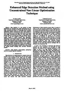
2 Step Edge Detection We use the notation P (i; j ) to denote the gray level of the pixel at location (i; j ) where i = 1; 2;


; N; j = 1; 2;


; M . At each image pixel P (i; j ), we de ne a 9  9 mask centered at pixel location (i; j ). For pixels on the image boundary, we construct their masks assuming that the image is wrapped around at the boundaries. The 9  9 mask centered at pixel P (i; j ) consists of nine SO pixels. The central SO pixel is denoted as P (2) (i; j ). Obviously, P (2) (i; j ) has two pairs of diagonally neighboring SO pixels which constitute the set ND and two pairs directly neighboring SO pixels which constitute the set N4. Depending on their locations, these SO pixels are denoted as P (2)(i + r; j + t) where ?1  r; t  1. We compute the weighted average of the gray level values of the 3  3 FO pixels within a SO pixel and regard the weighted average to be the gray level value of the SO pixel. We illustrate the procedure for computing the weighted average by considering the SO pixel P (2)(i ? 1; j + 1) shown in Fig. 2.1. The set of weights fa1; a2; a3; a4; a5g used in the weighted average are depicted in Fig. 2.2(a). The FO pixels in P (2) (i ? 1; j + 1) with the same weight are seen to be equidistant from P (i; j ) in the sense of the D4 (i.e. Manhattan) distance measure (Gonzalez and Woods, 1992). We require the weights fa1 ; a2; a3; a4; a5g to satisfy the following conditions: (i) a1 + 2a2 + 3a3 + 2a4 + a5 = 1; ai  0; i = 1; 2; 3; 4; 5: 4

(ii) fa1 ; a2; a3; a4; a5g is a linearly decreasing sequence and has a ratio relation as shown in Fig. 2.2(a). In Fig. 2.2(a), the numbers f4; 5; 6; 7; 8g on the horizontal axis denote the fact that the pixels with weight a1 are 4 units away from P (i; j ) and so on. The distance measure used is the D4 (i.e. Manhattan) distance measure. Condition (i) ensures that the weights are positive and normalized. Condition (ii) ensures that the weights decrease linearly with increasing Manhattan distance from pixel P (i; j ). These two conditions actually correspond to the triangular kernel density function used in statistical kernel smoothing techniques. For a detailed discussion on various smoothing kernels we refer the interested reader to the recent book by Wand and Jones (1995). We impose an additional constraint that the hypotenuse of the right-angled triangle shown in Fig. 2.2(a) intersect with the horizontal axis at point 9. This denotes the fact that pixels at Manhattan distance of 9 or greater from pixel P (i; j ) lie outside the neighborhood of interest. A unique weight sequence fa1; a2; a3; a4; a5g which satis es all the above requirements can be then determined and is given by: fa1; a2; a3; a4; a5g = f5=27; 4=27; 3=27; 2=27; 1=27g (2.1) The same weights are used for the other SO pixels 2 ND ; namely P (2)(i ? 1; j ? 1), P (2) (i +1; j ? 1) and P (2) (i + 1; j + 1). Consider the weights fb1; b2; b3g (shown in Fig. 2.2(b)) for the SO pixel P (2) (i ? 1; j ) (shown in Fig. 2.1). We require that the weights satisfy the conditions: (i) 3
(b1 + b2 + b3 ) = 1; bi  0; i = 1; 2; 3 (ii) The weights decrease linearly with increasing Manhattan distance from the pixel P (i; j ). (iii) The hypotenuse of the right-angled triangle shown in Fig. 2.2 (b) intersects the horizontal axis at point 5. The rationale behind these conditions is the same as that cited for the weights fai ; 1  i  5g. A unique solution satisfying all the above conditions is given by:

fb1; b2; b3g = f1=6; 1=9; 1=18g 5

(2.2)

b3

b3

b3

a3

a4

a5

P (2)(i ? 1; j ? 1) b2

b2

b2

a2

a3

a4

b1

b1

b1

a1

a2

a3

P (2)(i; j ? 1)

P (i; j )

P (2)(i; j + 1)

P (2)(i + 1; j + 1)

Figure 2.1: The 9  9 mask centered at pixel P (i; j ) as a union of nine SO pixels. Weights fa1; a2; a3; a4; a5g and fb1; b2; b3g are used in the diagonally neighboring SO pixels and in the directly neighboring SO pixels respectively. The same weights are used in other SO pixels 2 N4; namely, P (2)(i; j ? 1), P (2) (i + 1; j ) and P (2) (i; j + 1). Given the weights, the gray levels of the SO pixels P (2) (i ? 1; j + 1) and P (2) (i ? 1; j ) can be obtained thus:

P (2)(i ? 1; j + 1) = a1P (i ? 2; j + 2) + a2[P (i ? 2; j + 3) + P (i ? 3; j + 2)] +a3 [P (i ? 2; j + 4) + P (i ? 3; j + 3) + P (i ? 4; j + 2)] +a4 [P (i ? 3; j + 4) + P (i ? 4; j + 3)] + a5 P (i ? 4; j + 4)

(2.3)

P (2)(i ? 1; j ) = b1[P (i ? 2; j ? 1) + P (i ? 2; j ) + P (i ? 2; j + 1)] +b2[P (i ? 3; j ? 1) + P (i ? 3; j ) + P (i ? 3; j + 1)] +b3[P (i ? 4; j ? 1) + P (i ? 4; j ) + P (i ? 4; j + 1)]

(2.4)

6

HHH H a1

4

HHH HH HHH a2

5

a3

6

a4

ZZ ZZ ZZ (b) ZZ Z b1 b2 b3 ZZ Z

(a)

HHH a5 HH H9 7 8

2

3

4

5

Figure 2.2: Weights fa1 ; a2; a3; a4; a5g and fb1; b2; b3g satisfy the ratio relations as depicted in (a) and (b) respectively. The gray levels of other ND and N4 SO pixels can be obtained similarly. Intuitively, the dierences [P (2)(i ? 1; j +1) ? P (2)(i +1; j ? 1)], [P (2) (i ? 1; j ? 1) ? P (2)(i +1; j +1)],[P (2)(i ? 1; j ) ? P (2)(i +1; j )] and [P (2) (i; j ? 1) ? P (2) (i; j + 1)] can be looked upon as measures of the intensity discontinuity at pixel P (i; j ). If there is no step edge pixel in the 9  9 mask centered at pixel P (i; j ), then all of the aforementioned dierences could be expected to be small; on the other hand, if P (i; j ) is a step edge pixel, then some of them could be expected to be large. However, two other factors need to be considered as well; one is the variation of the underlying image intensity function in the 9  9 mask and the other is the variation of the gray levels caused by possible noise in the image. Intuitively, the variation of the intensity function along a direction can be measured by its rst order directional derivatives. For the direction from P (i + 3; j ? 3) to P (i ? 3; j + 3), we use

D(i ? 1; j + 1) = (d1 + d2)=2

(2.5)

to estimate the rst order directional derivative where

d1 =4 31 [P (i ? 4; j + 3) + P (i ? 4; j + 4) + P (i ? 3; j + 4)] ? 31 [P (i ? 3; j + 2) + P (i ? 2; j + 2) + P (i ? 2; j + 3)]

d2 =4 31 [P (i + 2; j ? 3) + P (i + 2; j ? 2) + P (i + 3; j ? 2)] ? 31 [P (i + 3; j ? 4) + P (i + 4; j ? 4) + P (i + 4; j ? 3)]

(2.6)

Here, d1 and d2 can be regarded as the estimates of the rst order directional derivatives at P (i ? 3; j + 3) and P (i + 3; j ? 3) respectively and D(i ? 1; j + 1) is their average. The famous Lagrange's Mean Value Theorem in dierential calculus tells us that for a 1-D function f (x) and two points x1 < x2 , f (x2) ? f (x1) = f 0 ()(x2 ? x1) for some  2 [x1; x2] as long as f (x) is dierentiable in 7

the interval [x1; x2]. This is equivalent to saying that the variation of f (x) from x1 to x2 could be approximated by the derivative multiplied by the distance between those two points. We de ne D (i ? 1; j ? 1) = 25 6
D(i ? 1; j ? 1) D(i ? 1; j + 1) = 25 6
D(i ? 1; j + 1) D(i ? 1; j ) = 38
D(i ? 1; j ) (2.7) D(i; j ? 1) = 83
D(i; j ? 1) D(i ? 1; j ? 1); D(i ? 1; j + 1); D(i ? 1; j ) and D(i; j ? 1) are used to measure the variation of the intensity function along the directions from P (i +3; j +3) to P (i ? 3; j ? 3), from P (i +3; j ? 3) to P (i ? 3; j + 3), from P (i + 3; j ) to P (i ? 3; j ) and from P (i; j + 3) to P (i; j ? 3) respectively. We refer to them as correction terms. The multiplicative factors of 256 and 83 are chosen such that the value of the edge detection criterion equals to zero when the intensity function is linear and when no edges exist at pixel (i; j ). In other words, the linear variation of the intensity function is eliminated from the edge detection process. The derivation of these two multiplicative factors is given in the Appendix. We de ne

1 2 3 4

4 (2) = P (i ? 1; j + 1) ? P (2)(i + 1; j ? 1) ? D(i ? 1; j + 1)

4 (2) = P (i ? 1; j ) ? P (2)(i + 1; j ) ? D(i ? 1; j )

4 (2) = P (i ? 1; j ? 1) ? P (2)(i + 1; j + 1) ? D(i ? 1; j ? 1) 4 (2) = P (i; j ? 1) ? P (2)(i; j + 1) ? D(i; j ? 1)

(2.8)

f1; 2; 3; 4g can all be expected be very small if there is no step edge in the 9  9 mask centered at P (i; j ). Since in reality, the gray levels are usually contaminated by noise, we have to consider the variation caused by the noise as well. We assume that the observed gray levels in the image are a realization of the following model:

P (i; j ) = g(i; j ) + n(i; j ); i = 1; 2;


; N; j = 1; 2;


; M where fg (i; j )g are the true gray levels and fn(i; j )g are independent and identically distributed (i.i.d) noise samples with zero mean and variance  2. With some simple algebraic manipulations (detailed in the Appendix), we can show that

std(1) = std(3) = 2:6202 8

std(2) = std(4) = 1:7951

(2.9)

where std(i ) denotes the standard deviation of i . We de ne

i i

4 = i=2:6202; for i = 1; 3

4 = i=1:7951; for i = 2; 4

(2.10)

If there is no edge pixel in the 9  9 mask centered at P (i; j ), then by the Central Limit Theorem in statistics (Bhattacharya and Johnson, 1977), f1 ; 2; 3; 4g are all approximately normally distributed with means zero and variances  2 since each of them is a linear combination of 18 observed gray levels. We then de ne MP (i;j) =4 maxfj1j; j2j; j3j; j4jg (2.11) as the step edge detection criterion. The statistical test corresponding to MP (i;j ) can be formulated as

P (MP (i;j) > C ()) =  , 1 ? [P (j1j < C ())]4 =  , P (j1j < C ()) = (1 ? )1=4 , C () = Z[1+(1?)1=4]=2
 where Z[1+(1?)1=4 ]=2 is the [1 + (1 ? )1=4]=2 percentile of the standard normal distribution. Statistically speaking, when there is no edge pixel in the 9  9 mask centered at pixel P (i; j ) and when  is very small, MP (i;j ) has little chance of exceeding C (). In other words, if MP (i;j ) is larger than C (), then we have sucient reason to conclude that there are edge pixels in the 9  9 mask. In such cases, we ag P (i; j ) as a step edge pixel. Thus, C () can be used as the threshold value for MP (i;j ) . But in most applications, since we do not know the value of  , it has to be estimated from the image data. In the following discussion, we will suggest two estimators of  . The applicable threshold value for MP (i;j ) can then be computed as:

C () = Z[1+(1?)1=4]=2
^ where ^ is an estimator of  . 9

(2.12)

Table 2.1: Several signi cance levels  and their corresponding [1 + (1 ? )1=4]=2 values and Z[1+(1?)1=4 ]=2 values. The notation Ae ? B denotes A  10?B .

 5.0e-01 4.5e-01 4.0e-01 3.5e-01 3.0e-01 2.5e-01 2.0e-01 1.5e-01 1.0e-01 5.0e-02 1.0e-02 5.0e-03 1.0e-03 5.0e-04 1.0e-04 5.0e-05

[1 + (1 ? )1=4]=2 Z[1+(1?)1=4 ]=2 0.9204482 1.408093 0.9305868 1.480175 0.9400559 1.555243 0.9489504 1.634761 0.9573456 1.720681 0.9653024 1.815839 0.9728708 1.924768 0.9800923 2.055659 0.9870019 2.226268 0.9936293 2.490915 0.9987453 3.022202 0.9993738 3.226681 0.9998750 3.662164 0.9999375 3.836061 0.9999875 4.214791 0.9999937 4.368675

 1.0e-05 5.0e-06 1.0e-06 5.0e-07 1.0e-07 5.0e-08 1.0e-08 5.0e-09 1.0e-09 1.0e-10 1.0e-11 1.0e-12 1.0e-13 1.0e-14 1.0e-15 1.0e-16

[1 + (1 ? )1=4]=2 Z[1+(1?)1=4 ]=2 0.9999987 4.708129 0.9999994 4.847543 0.9999999 5.157701 0.9999999 5.286029 1.0000000 5.573271 1.0000000 5.692763 1.0000000 5.961456 1.0000000 6.073695 1.0000000 6.326984 1.0000000 6.673367 1.0000000 7.003303 1.0000000 7.318952 1.0000000 7.622118 1.0000000 7.905250 1.0000000 8.209103 1.0000000 In nite

Remark 2.1: Z[1+(1?)1=4]=2 depends on the signi cance level . Without confusion, we may sometimes refer to it as the threshold value. Table 2.1 lists several  values and their corresponding [1 + (1 ? )1=4]=2 values and Z[1+(1?)1=4]=2 values.

In the above hypothesis testing procedure, the probability of detecting a false edge at each pixel is . On the other hand, edges with jump magnitude less than 1:7951Z[1+(1?)1=4]=2
^ (edges with low SNR, c.f. equation (2.9)) could probably be missed. Thus Z[1+(1?)1=4 ]=2 works as a tuning parameter by which to balance missing-edge=false-edge possibilities. Although it is related to the con dence level , this relationship is only approximate because of the use of the Central Limit Theorem which provides an approximate normal distribution for a nite sample size (only 18 in our case). In typical applications, the threshold value still needs to be somewhat 10

heuristically adjusted. Theoretically, it is not dicult to establish the statistical consistency of the aforementioned edge detection procedure. Also, the missing-edge=false-edge probabilities both tend to zero with increasing spatial resolution of the image. We refer the interested readers to the related discussions in Qiu and Yandell (1995) for a more detailed treatment of this topic. A nature estimator of  is the sample standard deviation of the gray levels in the 9  9 mask centered at P (i; j ). But if there are edge pixels in the mask, this estimator performs poorly. We therefore propose to estimate  in the following manner: In each of the eight neighboring SO pixels, we compute the sample variance of the gray levels of its 3  3 FO pixels. These variances are denoted as s2 (i ? r; j ? t), where r; t = ?1; 0; 1, (r; t) 6= (0; 0). We de ne

^ (i; j ) = medianf (i; j ? 1);  (i ? 1; j ? 1);  (i ? 1; j );  (i ? 1; j + 1)g where

 (i; j ? 1)  (i ? 1; j ? 1)  (i ? 1; j )  (i ? 1; j + 1)

q [s2(i; j ? 1) + s2 (i; j + 1)]=2 q = [s2(i ? 1; j ? 1) + s2 (i + 1; j + 1)]=2 q = [s2(i ? 1; j ) + s2 (i + 1; j )]=2 q = [s2(i ? 1; j + 1) + s2 (i + 1; j ? 1)]=2

(2.13)

=

(2.14)

Obviously, each of  (i; j ? 1);  (i ? 1; j ? 1);  (i ? 1; j ) and  (i ? 1; j +1), which is derived from the SO pixel pair [P (2)(i; j ? 1); P (2)(i; j +1)]; [P (2)(i ? 1; j ? 1); P (2)(i +1; j +1)]; [P (2)(i ? 1; j ); P (2)(i +1; j )] and [P (2) (i ? 1; j + 1); P (2)(i + 1; j ? 1)] respectively, is a nature estimator of  . We assume that if P (i; j ) is an edge pixel, then at least one of the SO pairs cited above is such that one of the SO pixels in the pair is on one side of the edge and the other SO pixel is on the other side. Estimators of  based on the above SO pixel pairs will not be aected by the presence of edges in the 9  9 mask centered at pixel P (i; j ). In other words, ^ (i; j ) provides a good estimator of  whether or not there are edge pixels in the 9  9 mask centered at pixel P (i; j ). We term ^ (i; j ) as the zeroth-order estimator of  because the sample variance s2 (i ? r; j ? t) can be regarded as the residual mean squares when the sample mean is regarded as the estimator of the true FO pixel gray levels in the SO pixel P (2) (i ? r; j ? t). The sample mean is a zeroth-order estimator in the sense that it is a zeroth-order polynomial. Clearly, each of s2 (i ? r; j ? t); r; t = ?1; 0; 1; (r; t) 6= (0; 0), is a rough estimator of  2 because the sample mean is a rough estimator of the true FO pixel gray levels in the corresponding SO pixel. 11

A more accurate estimator of  can be constructed as follows: In each of the eight neighboring SO pixels P (2) (i ? r; j ? t), we perform a least-squares planar t and then obtain the residual mean squares s2 (i ? r; j ? t). After some algebraic manipulations (detailed in the Appendix), we have the following expression for s2 (i ? r; j ? t): (2.15) s2 (i ? r; j ? t) = 61 (Y 0 Y ? Y 0PX Y ) where Y is a 9  1 vector whose elements are the gray levels of the 3  3 FO pixels in P (2) (i ? r; j ? t) scanned in a row-major (i.e. raster-scan) fashion (i.e. left-to-right and top-to-bottom). The 9  9 matrix PX is given by:

2 66 8 66 5 66 66 2 66 5 66 1 PX = 18  66 2 66 66 ?1 66 66 2 66 ?1 4 ?4

5 5 5 2 2 2

2 5 8

5 2

2 2 ?1 2 ?1 5 2 2 2 2 5 ?1 2 ?1 ?4 5 2 ?1 ?1 2 2 ?1 2 ?1 2

3 ?1 ?4 7 7 ?1 ?1 77 7 ?1 2 777 7 2 ?1 77 7 2 2 2 2 77 7 5 ?1 2 5 777 7 ?1 8 5 2 77 7 2 5 5 5 775

?1 2 2 ?1 5 ?4 ?1 5

5

2

5

(2.16)

8

We then de ne

^(i; j ) = medianf(i; j ? 1); (i ? 1; j ? 1); (i ? 1; j ); (i ? 1; j + 1)g where

(i; j ? 1) (i ? 1; j ? 1) (i ? 1; j )  (i ? 1; j + 1)

q [s2 (i; j ? 1) + s2 (i; j + 1)]=2 q = [s2 (i ? 1; j ? 1) + s2 (i + 1; j + 1)]=2 q = [s2 (i ? 1; j ) + s2 (i + 1; j )]=2 q = [s2 (i ? 1; j + 1) + s2 (i + 1; j ? 1)]=2

(2.17)

=

We term ^ (i; j ) as the rst-order estimator of  . We summarize the step edge detection method discussed above in the following algorithm:

Step Edge Detection Algorithm 12

(2.18)

1. For every pixel, P (i; j ); i = 1; 2;


; N; j = 1; 2;


; M , consider the 9  9 mask centered at P (i; j ). Use equations (2.1){(2.4) to compute P (2) (i ? r; j ? t), where r; t = ?1; 0; 1 and (r; t) 6= (0; 0). 2. Use equations (2.5){(2.7) to compute D(i?1; j +1); D(i?1; j ); D(i?1; j ?1) and D(i; j ?1). 3. Use equations (2.8), (2.10) and (2.11) to compute the value of MP (i;j ) . 4. Use equations (2.13){(2.14) or (2.17){(2.18) to obtain an estimator of  and then use equation (2.12) to obtain a threshold value C (). In most practical applications, Z[1+(1?)1=4 ]=2 can be chosen between 7.5 and 10. 5. Compare MP (i;j ) with C (). If MP (i;j ) > C (), then P (i; j ) is agged as a step edge pixel.

We have the following remarks to make on our step edge detection technique:

Remark 2.2: In equations (2.3) and (2.4) we use the unequal weights given by equations (2.1) and (2.2) instead of equal weights because of the following considerations: If we use the unequal weights given by equations (2.1) and (2.2) in equations (2.3) and (2.4), then std(P (2)(i ? 1; j +1))  0:3572 and std(P (2) (i ? 1; j ))  0:36 . If we use equal weights in equations (2.3) and (2.4), then std(P (2)(i ? 1; j + 1)) = std(P (2)(i ? 1; j ))  0:3333. These standard deviation values indicate that the noise removal capability of the technique with equal weights or with unequal weights is almost the same. But the blurring eect with unequal weights will be much less than with equal weights. For a more detailed discussion on the selection of weights we refer the interested reader to Chapter 4, Section 4.3 in the book by Gonzalez and Woods (1992). Another consideration for using unequal weights instead of equal weights is to increase the accuracy of the detected edges. If we use equal weights, then pixels 3 units away (Manhattan distance) from the true edges could still be detected with large probability. If we use the unequal weights in the 9  9 window centered at P (i; j ) as we did in equations (2.3)-(2.4), the weighted centers of the SO pixels are closer to P (i; j ), thus improving the localization of the detected edges. Pixels about 2 units away from the true edges, in this case, would hardly be detected.

Remark 2.3: We recommend the use of the zeroth-order or the rst-order estimator of  in

equation (2.12). Higher order estimators of  could also be formulated and used but would involve a greater computational overhead. Our experimental results have shown that the rst-order estimator 13

provides enough accuracy for most applications because the least-squares plane provides a good t to the true image intensity surface in a small region where the image intensity function is continuous.

Remark 2.4: The 9  9 mask of P (i; j ) is the smallest size mask that contains non-overlapping

SO pixels that are eight-neighbors of the central SO pixel. This simpli es our theoretical analysis.

Remark 2.5: In the model, we assumed that noise samples n(i; j ) are independent and identically

distributed and have an identical variance  2. In many applications, however, the noise samples might be correlated and their variances may be a function of the spatial coordinates (i; j ) (i.e. non-stationary noise). In the latter case (i.e. non-stationary noise), our method should still work well since the estimators of the variance that we propose are locally constructed. We do use the assumption of independence of the noise samples in equation (2.9). If noises are correlated, the coecients in equation (2.9) would need to be modi ed accordingly where the modi cation depends on the pattern of correlation. For a detailed discussion on the estimation of spatial correlation we refer the interested reader to Cressie (1991). Comparing with some \traditional" edge detectors such as the Sobel, Roberts and Laplacian of Gaussian (LoG), our edge detection criterion has the following features: 1. The variation of the underlying intensity function is almost deleted from the edge detection criterion by using the correction terms. More speci cally, MP (i;j ) has the property that

8 > < C (i; j ) + h22 g00(i; j ), if the (i; j )th pixel is an edge pixel MP (i;j) ' > h2 00 : 2 g (i; j ), otherwise

where C (i; j ) denotes the step magnitude of the intensity function at pixel (i; j ) and h is the window width (i.e. window of size h  h). The eect of the variation of the underlying intensity function on the edge detection is re ected by the second order term h22 g 00(i; j ). For most other existing edge detectors, this eect is approximately hg 0(i; j )+ h22 g 00(i; j ). Thus the linear term hg 0(i; j ) has been eliminated from our edge detection criterion. 2. We consider four directions instead of only the x and y directions in the construction of the edge detection criterion. That makes the procedure more exible in its capability of dealing with the local smoothness of the image intensity function. 3. The correction terms result in the introduction of noise in edge detection process. This noisy eect is, however, greatly reduced by introducing the concepts of FO and SO pixels and by 14

using local smoothing in each SO. The variance of the noise in the gray level of each SO is about 1=9 the variance of the noise in each FO. The experimental results in the following section will clarify the above remarks.

3 Experimental Results for the Step Edge Detection Algorithm In this section, we present experimental results of our step edge detection algorithm when applied to gray scale intensity images. We also discuss the eects of various parameters on the performance of the algorithm. The gray scale image of size 512  512 pixels with a gray scale resolution of 8 bits per pixel shown in Fig. 3.1 was used for the purpose of testing our algorithm. We used our step edge detection algorithm to detect step intensity edges within this image. The output edge image is a binary image; if pixel P (i; j ) is agged as a step edge pixel, then we set its gray level value to 255 else we reset its gray level value to 0. Fig. 3.2 (a) { (d) shows the result of our algorithm with four dierent threshold values Z[1+(1?)1=4 ]=2 = 3:5; 7:5; 10; 15 using the rst-order estimator of . These results show that the step edge images are best detected with the threshold values in the range [7:5; 10]. If the threshold value is too small, then many false edges are detected. On the other hand, if the threshold value is too large, then many true edges are missed. Based on a number of experiments, we recommend threshold values between 7:5 and 10. Fig. 3.3 (a){(d) shows two other gray scale images and the corresponding edge images wherein the step edges were detected with a threshold value of 8. Fig. 3.1 goes here Fig. 3.2 (a), (b), (c), (d) goes here Fig. 3.3 (a), (b), (c), (d) goes here We also experimented with the zeroth-order estimator of  and the results are shown in Fig. 3.4 (a){(d). The experimental results show that the threshold values need to be smaller in this case. The reason behind this phenomenon is that the zeroth-order estimator of  is usually larger than the rst-order estimator because the former includes a greater variation of the image intensity function. Consequently the zeroth-order estimator is not as accurate as the rst-order estimator resulting in the detection of several false edges. 15

Fig. 3.4 (a), (b), (c), (d) goes here Next we study the eect of exclusion of the correction terms D(:; :) from equations (2.8). The rst-order estimator of  is used. Accordingly the formulas for i in equation (2.10) replaced by the following ones:

i = i =0:5051; for i = 1; 3 i = i =0:5092; for i = 2; 4 The results are shown in Fig. 3.5 (a){(d). From our experimental results, we make the following observations: Our rst observation that very large threshold values need to be chosen. This is a result of the fact that we do not exclude the variations of the intensity function from our criterion MP (i;j) as was done previously thus resulting in a larger value for MP (i;j) . The other observation is that the detected edges are very thick. Fig. 3.5 (a), (b), (c), (d) goes here Finally, we compare the performance of our edge detection technique and two \classical" edge detectors: the Sobel and LoG. Fig. 3.6 (a) shows a synthesized gray scale image. Pixels on scan lines 1-86 have a gray level value of 155 whereas those on scan lines 87-172 have a gray level value of 165. From scan line 173 to line 212, the gray level values decrease linearly and are described by the linear function 255 ? 6  (i ? 172) where i is the scan line number. The image between the scan lines 213 and 512 is divided into two portions. The left portion consists of 8 sections where the gray level values in each section are identical. The gray level values of adjacent sections alternate between 155 and 165. In the right portion, the gray level values on scan lines 213-312 are 100, on scan lines 313-412 are 75 and on scan lines 413-512 are 100 again. White noise from a uniform distribution U (?10; 10) is added to the gray level value of each pixel in the right portion. Fig. 3.6 (b) shows the result of the Sobel edge detector. In the top portion of the image, it misses the edge between scan lines 86-87 and falsely detects the region between scan lines 173-212. In the region between scan lines 173-212, the gray levels have a steep linear trend, but no edges exist. Since the Sobel edge detector does not exclude the linear trend of the underlying intensity function 16

from edge detection process, it cannot overcome this false-edge detection problem and also detect the true edge between scan lines 86-87 at the same time. In the left portion of the bottom half of the image, there are two diagonal edge boundaries, one vertical edge boundary and one horizontal edge boundary; all of which have the same intensity step magnitudes. However, as we can be seen from Figure 3.6 (b), the Sobel detector could detect two diagonal edge boundaries whereas it misses the other two edge boundaries. The reason behind this is that the Sobel operator only considers two orthogonal directions (x and y ) in the edge detection process. The Sobel operator detects the true edge boundaries in the noisy portion (i.e. right lower portion) of the image but also several noisy edge pixels as well. Fig. 3.6 (c) shows the edges detected by the LoG operator. The LoG operator suers from some of the same drawbacks as the Sobel operator. Note that although the false-edge detection problem in the region between scan lines 173-212 has been somewhat alleviated, the true edge between scan lines 86-87 has been missed. The LoG operator misses most of the edge boundaries in the noisy portion of the image although it suppresses the noisy edge pixels in doing so. It also does not detect all the eight edge boundaries in the left lower portion of the image. The result of the proposed edge detection technique is shown in Fig. 3.6 (d). We can see that the false-edge detection problem due to the steep linear trend in image intensity values has been alleviated. All the true step edges in the upper portion of the image are detected. Also, all the 8 edge boundaries at various orientations in the left lower portion of the image are detected. In the noisy portion of the image, the true edge pixels and fewer noisy pixels are detected. Our method however also has its limitations. One, is that the detected edges are quite thick. This is the price we pay for the use of larger windows (9  9) in order to eliminate the eect of the linear variation of the intensity function. The proposed technique also detects noisy edge pixels. These limitations can be overcome by postprocessing techniques that thin the detected edges, connect fragmented edges and eliminate scattered noisy edge points. A few such postprocessing techniques have been described in Chapter 7, Section 7.2 in the book by Gonzalez and Woods (1992). Fig. 3.6 (e) shows the results after the use of the postprocessing procedures proposed by Qiu and Yandell (1995) (these procedures are described in the Appendix) to the results depicted in Fig. 3.6 (d). We can see the improvement in results. The postprocessing results around the intersections of edge boundaries are still not quite satisfactory. This is partly due to the inherent limitations of the postprocessing procedures. For a more detailed discussion on this issue, we refer the interested 17







@
@
@
@
@

s?1 s

@

s+1

Figure 4.1: Local cross section of an image intensity surface where pixel s is an ideal roof edge pixel. reader to the recent work of Qiu and Yandell (1995). Fig. 3.6 (a), (b), (c), (d), (e) goes here

4 Roof Edge Detection In this section, we discuss the extension of our step edge detection technique to roof edge detection. As already mentioned, a roof edge signi es a discontinuity in the rst derivative but continuity in the value of the image intensity function. Fig. 4.1 shows the cross section of the image intensity surface in the vicinity of a roof edge. Pixel s in Fig. 4.1 is an ideal roof edge pixel. From Fig. 4.1, we make the following observations: (1) jg 0(s + 1) ? g 0(s ? 1)j is large i.e. g 0(
) has a step discontinuity at s. Here, g 0(
) denotes the rst order derivative of the intensity function g (
). (2) g 0(s ? 1)  g 0(s)  g 0(s + 1). Furthermore, g 0(s ? 1) + g 0(s + 1) ? 2g 0(s) = 0 where g 0(s) is de ned as g 0(s) = lim
s!0 [g (s +
s) ? g (s ?
s)]=2
s. The above two observations are the basis of our roof edge detection algorithm. At a given pixel location P (i; j ), we consider the 9  9 mask centered at that pixel (c.f. Fig. 2.1) consisting of nine SO pixels P (2) (i + s; j + t); s; t = ?1; 0; 1. As in the case of step edge detection, we consider four directions: the two diagonal directions and the two orthogonal directions along 18

the image rows and columns. For the direction from P (i + 3; j ? 3) to P (i ? 3; j + 3) , we use d1 and d2 which are computed as shown in equations (2.6) to estimate the directional derivatives at pixels P (i ? 3; j + 3) and P (i + 3; j ? 3) respectively. Similarly, we compute d3 =4 13 [P (i ? 1; j ) + P (i ? 1; j + 1) + P (i; j + 1)] ? 31 [P (i; j ? 1) + P (i + 1; j ? 1) + P (i + 1; j )] (4.1) which is used as an estimator of the rst order directional derivative at pixel P (i; j ). An additional correction term is used to subtract the variation of the rst order directional derivative of the image intensity function along that direction. Let c1 =4 31 [P (i ? 4; j + 3) + P (i ? 4; j + 4) + P (i ? 3; j + 4) +P (i ? 3; j + 2) + P (i ? 2; j + 2) + P (i ? 2; j + 3)] ? 32 [P (i ? 4; j + 2) + P (i ? 3; j + 3) + P (i ? 2; j + 4)] c2 =4 31 [P (i + 2; j ? 3) + P (i + 2; j ? 2) + P (i + 3; j ? 2)

+P (i + 3; j ? 4) + P (i + 4; j ? 4) + P (i + 4; j ? 3)] (4.2) ? 32 [P (i + 2; j ? 4) + P (i + 3; j ? 3) + P (i + 4; j ? 2)] Then c1 and c2 can be regarded as the estimators of the second order directional derivatives of the image intensity function at P (i ? 3; j + 3) and P (i + 3; j ? 3) respectively. Also c =4 c1 +2 c2 (4.3) can be used as an estimator of the second order directional derivative at P (i; j ). We could choose the multiplicative factors as we did in equations (2.7) to delete the quadratic variation of the image intensity function from the process of roof edge detection. Given the complexity of this computation, we suggest using 5 as the multiplicative factor which is the Manhattan distance from P (i ? 3; j + 3) to P (i + 3; j ? 3). We then de ne

1 =4 d1 ? d2 ? 5c

(4.4)

1 =4 d1 + d2 ? 2d3

(4.5)

We similarly de ne the corresponding quantities 2 ; 3; 4 and 2; 3; 4 along the other three directions. Clearly, the quantities f1; 2; 3 ; 4g are a measure of observation (1) made at at the beginning of this section. Similarly, the quantities f 1; 2; 3; 4g are a measure of observation (2). 19

If there are no step edge pixels and roof edge pixels in the 9  9 mask centered at pixel P (i; j ), then 1 ; 2 ; 3 and 4 are all approximately normally distributed with zero means and standard deviations  . From equations (2.6) and (4.2)-(4.4), we can easily compute the value of  to be  = 5:1316. By the same reasoning as in the case of step edge detection, if there is some i which satis es the relation jij > Z1?=2
5:1316^ (4.6) then we have sucient reason to believe that P (i; j ) is a roof edge pixel. However, if there are some step edge pixels in the 9  9 mask of P (i; j ), they too could result in large values for some of the i 's. We therefore need to check an additional condition before making a nal decision whether or not P (i; j ) is a roof edge pixel. The other condition is derived from the quantities f 1; 2; 3; 4g. As pointed out earlier, if P (i; j ) is a roof edge pixel, then some of f ig's should be small (corresponding to observation (2) that g 0(s ? 1) + g 0(s + 1) ? 2g 0(s) = 0). From equations (2.6), (4.1) and (4.5), we can easily show that std( i) = 2; i = 1; 2; 3; 4. That i is small can be de ned statistically as follows: j ij  Z1?=2
2^ (4.7) At P (i; j ), let us suppose that fi1 ; i2 ;


; ir g  f1 ; 2; 3; 4g contains the  values which satisfy condition (4.6) where r  4. Then we test the corresponding values f i1 ; i2 ;


; ir g using condition (4.7). If at least one of the values satis es condition (4.7), then we decide that P (i; j ) is a roof edge pixel. We summarize our roof edge detection technique in the following algorithm.

Roof Edge Detection Algorithm 1. For a given pixel P (i; j ); 1  i  N; 1  j  M , consider the 9  9 mask centered at that pixel. Compute f1 ; 2; 3; 4g and f 1; 2; 3; 4g using equations (2.6) and (4.1){(4.5). 2. Consider the pairs (1; 1); (2; 2); (3; 3) and (4 ; 4) one at a time. If at least one of them satis es both conditions (4.6) and (4.7), then P (i; j ) is agged as a roof edge pixel.

We have tested our roof edge detection algorithm on some synthetic images. One such image is shown in Fig. 4.2 (a). Pixels that lie on the horizontal line in the center of the image are assigned a gray level value of 255. The gray level values decrease linearly to zero along the columns of the image on either side of the horizontal line. Thus we have a roof edge along the horizontal line in 20

the center of the image. The resulting edge image from the roof edge detection algorithm is shown in Fig. 4.2 (b). As can be seen, the roof edge is completely detected. Fig. 4.2 (a), (b) goes here

5 Conclusions We have proposed algorithms for step edge detection and roof edge detection in this paper. Our algorithms combine local smoothing with statistical hypothesis testing to detect step and roof edges in gray scale images. We have used some locally-weighted averaging procedures to remove the noise and derived the appropriate edge detection criteria thereby giving our algorithms the ability to detect edges in noisy images as well. At each pixel location P (i; j ), we consider a 9  9 mask centered at that pixel. This mask is regarded as a union of nine SO pixels with four pairs of SO pixels along each of the four directions { horizontal, vertical and the two diagonal directions. Our algorithms detect the edges along these four directions and are very exible with regard to the local smoothness properties of the image intensity function. Another important feature of our algorithms is their ability to eliminate the eect of the linear variation of the image intensity function from the process of edge detection which is seen to improve the results of the edge detection process. The proposed edge detection technique, however, has room for improvement. First, we have used a xed-size 9  9 mask all throughout. In certain applications, masks with variable or adaptable sizes may be more appropriate. In some planar regions of the image intensity function, we could use large-size masks whereas in highly textured regions, the sizes of the masks could be small. Secondly, in detecting an edge at P (i; j ), we use only the pixels in its 9  9 mask in making a decision, i.e. no other information is used. In many cases, some additional information, typically of a contextual nature, may be useful for edge detection. Thirdly, as in the case of some other local smoothing lters, the detected edges resulting from our algorithms may be thick and fragmented at some places. This would call for some global smoothing/sharpening techniques (Acton and Bovik, 1992; Bhandarkar et al., 1994; Tan et al., 1989; 1991) to be used in conjunction with the algorithms presented here. We will address these issues in our future research.

Acknowledgments The authors thank Ms. Peiying Jia, Department of Biological and Agricul21

tural Engineering, University of Georgia, who helped them with the coding and testing of their algorithms. The authors thank the editor and the anonymous referees whose insightful comments greatly improved the paper.

References Acton, S.T., and Bovik, A.C. (1992). Anisotropic edge detection using mean eld annealing, Proc. IEEE Intl. Conf. Acous. Speech Sig. Proc. II, 393-396. Ashkar, G.P., and Modestino, J.W. (1978). The contour extraction problem with biomedical applications. Comp. Graph. Img. Proc. 7, 331-355. Bhandarkar, S.M., Zhang, Y., and Potter, W.D. (1994). An edge detection technique using genetic algorithm-based optimization. Pattern Recognition. 27(9), 1159-1180. Bhattacharya, G.K., and Johnson, R.A. (1977). Statistical Concepts and Methods. John Wiley and Sons Inc., New York, NY. Canny, J.F. (1986). A computational approach to edge detection, IEEE Trans. Patt. Anal. Mach. Intell. 8(6), 679-698. Chen, M.H., Lee, D., and Pavlidis, T. (1991). Residual analysis for feature detection. IEEE Trans. Patt. Anal. Mach. Intell. 13(1), 30-40. Cressie, N. (1991). Statistics for Spatial Data. John Wiley Inc., New York, NY. Dickey, F.M., and Shanmugam, K.S. (1977). Optimum edge detection lter. Appl. Optics. 16(1), 145-148. Gonzalez, R.C., and Woods, R.E. (1992). Digital Image Processing. Addison-Wesley Pub. Co. Reading MA. Hansen, F.R., and Elliot, H. (1982). Image segmentation using simple Markov eld models. Comp. Graph. Img. Proc. 20, 101-132. Haralick, R.M. (1984). Digital step edges from zero crossing of second directional derivatives. IEEE Trans. Patt. Anal. Mach. Intell. 6(1), 58-68. 22

Huang, J.S., and Tseng, D.H. (1988). Statistical theory of edge detection. Comp. Vis. Graph. Img. Proc. 43, 337-346. Lee, D., and Wasilkowski, G.W. (1991). Discontinuity detection and thresholding { a stochastic approach. Proc. IEEE Conf. Comp. Vis. Patt. Recog. 208-214. Marr, D., and Hildreth, E. (1980). Theory of edge detection. Proc. Royal Soc. London. B 207, 187-217. Martelli, A. (1976). An application of heuristic search to edge and contour detection. Comm. ACM. 19(2), 73-83. Montanari, U. (1971). On the optimal detection of curves in noisy pictures. Comm. ACM. 14(5), 335-345. Nalwa, V., and Binford, T. (1986). On detecting edges. IEEE Trans. Patt. Anal. Mach. Intell. 8(6), 699-714. Peli, T., and Malah, D. (1982). A study of edge detection algorithms. Computer Graphics and Image Processing. 20, 1-21. Perona, P., and Malik, J. (1990). Scale space and edge detection using anisotropic diusion. IEEE Trans. Patt. Anal. Mach. Intell. 12(7), 629-639. Qiu, P., and Yandell, B. (1995). Jump detection in regression surfaces. Technical Report 948. Dept. of Statistics, University of Wisconsin-Madison, Madison, WI 53706, USA. Saint-Marc, P., Chen, J., and Medioni, G. (1991). Adaptive smoothing: a general tool for early vision, IEEE Trans. Patt. Anal. Mach. Intell. 13(6), 514-529. Sarkar, S.S., and Boyer, K.L. (1990). On optimal in nite impulse response edge detection lters. IEEE Trans. Patt. Anal. Mach. Intell. 13, 1154-1171. Shen, J., and Castan, S. (1992). An optimal linear operator for step edge detection. CVGIP: Graph. Models Img. Proc. 54(2), 112-133. Sinha, S.S., and Schunk, B.G. (1992). A two-stage algorithm for discontinuity-preserving surface reconstruction. IEEE Trans. Patt. Anal. Mach. Intell. 14, 36-55. 23

Tan, H.L., Gelfand, S.B., and Delp, E.J. (1989). A comparative cost function approach to edge detection. IEEE Trans. Sys. Man Cyber. 19(6), 1337-1349. Tan, H.L., Gelfand, S.B., and Delp, E.J. (1991). A cost minimization approach to edge detection using simulated annealing. IEEE Trans. Patt. Anal. Mach. Intell. 14(1), 3-18. Torre, V., and Poggio, T.A. (1986). On edge detection. IEEE Trans. Patt. Anal. Mach. Intell. 8(2), 147-163. Wand, M.P., and Jones, M.C. (1995). Kernel Smoothing. Chapman & Hall, London, UK.

24

APPENDIX 1. Derivation of the multiplicative factors in equations (2.7) The multiplicative factors in equations (2.7) are chosen such that the linear variation of the intensity function is deleted from the edge detection criterion. Let us assume that the intensity function has a linear form a  i + b  j + c at each pixel (i; j ), where a; b and c are constants. We then choose the multiplicative factors such that MP (i;j ) = 0. Without loss of generality, the case of MP (5;5) is discussed in the following example: In the 9  9 mask of P (5; 5), according to equations (2.3)-(2.4), 5 P (3; 7) + 4 [P (3; 8) + P (2; 7)] + 3 [P (3; 9) + P (2; 8) + P (1; 7)] P (2)(5 ? 1; 5 + 1) = 27 27 27 2 1 + 27 [P (2; 9) + P (1; 8)] + 27 P (1; 9) 5 (3a + 7b + c) + 4 (5a + 15b + 2c) + 3 (6a + 24b + 3c) + = 27 27 27 2 (3a + 17b + 2c) + 1 (a + 9b + c) 27 27 70 20 = 9 a+ 9 b+c

5 P (7; 3) + 4 [P (8; 3) + P (7; 2)] + 3 [P (9; 3) + P (8; 2) + P (7; 1)] P (2)(5 + 1; 5 ? 1) = 27 27 27 1 2 + 27 [P (9; 2) + P (8; 1)] + 27 P (9; 1) 5 (7a + 3b + c) + 4 (15a + 5b + 2c) + 3 (24a + 6b + 3c) + = 27 27 27 2 (17a + 3b + 2c) + 1 (9a + b + c) 27 27 70 20 = 9 a+ 9 b+c

From equations (2.5) and (2.6),

D(5 ? 1; 5 + 1) = 61 [(P (1; 8) + P (1; 9) + P (2; 9)) ? (P (2; 7) + P (3; 7) + P (3; 8)) +(P (7; 2) + P (7; 3) + P (8; 3)) ? (P (8; 1) + P (9; 1) + P (9; 2))] = 16 [(4a + 26b + 3c) ? (8a + 22b + 3c) + (22a + 8b + 3c) ? (26a + 4b + 3c)] = 4 (b ? a) 3

25

In equations (2.7), let us assume that

D(5 ? 1; 5 + 1) = m1
D(5 ? 1; 5 + 1) where m1 is the rst multiplicative factor. Then from equations (2.8)

1 = P (2)(5 ? 1; 5 + 1) ? P (2)(5 + 1; 5 ? 1) ? D (5 ? 1; 5 + 1) = ( 20 a + 70 b + c) ? ( 70 a + 20 b + c) ? 4 m1(b ? a) 9 9 9 9 3

If we let 1 = 0, then m1 = 256 . Hence the rst multiplicative factor should be chosen as 256 in order to make MP (5;5) = 0. Similarly,

P (2)(5 ? 1; 5) = 16 [P (3; 4) + P (3; 5) + P (3; 6)] + 19 [P (2; 4) + P (2; 5) + P (2; 6)] + 1 [P (1; 4) + P (1; 5) + P (1; 6)] 18 = 1 (9a + 15b + 3c) + 1 (6a + 15b + 3c) + 1 (3a + 15b + 3c) 6 9 18 15 7 = 3 a + 3 b + c;

P (2)(5 + 1; 5) = 61 [P (7; 4) + P (7; 5) + P (7; 6)] + 19 [P (8; 4) + P (8; 5) + P (8; 6)] + 1 [P (9; 4) + P (9; 5) + P (9; 6)] 18 1 (27a + 15b + 3c) = 16 (21a + 15b + 3c) + 91 (24a + 15b + 3c) + 18 15 b + c; = 23 a + 3 3

D(5 ? 1; 5) = 61 [(P (1; 4) + P (1; 5) + P (1; 6)) ? (P (3; 4) + P (3; 5) + P (3; 6)) +(P (7; 4) + P (7; 5) + P (7; 6)) ? (P (9; 4) + P (9; 5) + P (9; 6))] = 1 [(3a + 15b + 3c) ? (9a + 15b + 3c) + (21a + 15b + 3c) ? (27a + 15b + 3c)] 6 = ?2a If we denote the second multiplicative factor as m2 and we let 2 = 0, then from equations (2.7) and (2.8), we have m2 = 38 . 26

2. Derivation of equations (2.9) From equations (2.5), (2.7) and (2.8),

1 = P (2)(i ? 1; j + 1) ? P (2)(i + 1; j ? 1) ? D (i ? 1; j + 1) = P (2)(i ? 1; j + 1) ? P (2) (i + 1; j ? 1) ? 25 6
D(i ? 1; j + 1)

25 d ? 25 d = P (2)(i ? 1; j + 1) ? P (2) (i + 1; j ? 1) ? 12 1 12 2 25 d ] ? [P (2) (i + 1; j ? 1) + 25 d ] = [P (2)(i ? 1; j + 1) ? 12 1 12 2 25 (2) Clearly, P (2) (i ? 1; j + 1) ? 25 12 d1 and P (i + 1; j ? 1) + 12 d2 are independent and have the same variances. So 25 d ]: V ar(1) = 2V ar[P (2)(i ? 1; j + 1) ? 12 1

From equations (2.3) and (2.6),

P (2)(i ? 1; j + 1) ? 25 12 d1

So

5 P (i ? 2; j + 2) + 4 [P (i ? 2; j + 3) + P (i ? 3; j + 2)] = 27 27 3 + [P (i ? 2; j + 4) + P (i ? 3; j + 3) + P (i ? 4; j + 2)] 27 2 [P (i ? 3; j + 4) + P (i ? 4; j + 3)] + 1 P (i ? 4; j + 4) + 27 27 25 ? 36 [P (i ? 4; j + 3) + P (i ? 4; j + 4) + P (i ? 3; j + 4)] + 25 36 [P (i ? 3; j + 2) + P (i ? 2; j + 2) + P (i ? 2; j + 3)] 5 + 25 )P (i ? 2; j + 2) + ( 4 + 25 )[P (i ? 2; j + 3) + P (i ? 3; j + 2)] = ( 27 36 27 36 3 + 27 [P (i ? 2; j + 4) + P (i ? 3; j + 3) + P (i ? 4; j + 2)] +( 2 ? 25 )[P (i ? 3; j + 4) + P (i ? 4; j + 3)] + ( 1 ? 25 )P (i ? 4; j + 4) 27 36 27 36 25 d ] V ar[P (2)(i ? 1; j + 1) ? 12 1

= [( 5 + 25 )2 + 2( 4 + 25 )2 + 3( 3 )2 + 2( 2 ? 25 )2 + ( 1 ? 25 )2] 2 27 36 27 36 27 27 36 27 36 2 = 3:4326 Hence

V ar(1) = 6:8652 2 std(1 ) = 2:6202 27

From equations (2.7) and (2.8),

2 = P (2)(i ? 1; j ) ? P (2)(i + 1; j ) ? D(i ? 1; j ) = P (2)(i ? 1; j ) ? P (2)(i + 1; j ) ? 8
D(i ? 1; j ) 3

= P (2)(i ? 1; j ) ? 94 [P (i ? 4; j ? 1) + P (i ? 4; j ) + P (i ? 4; j + 1)] + 49 [P (i ? 2; j ? 1) + P (i ? 2; j ) + P (i ? 2; j + 1)] ?P (2)(i + 1; j ) + 94 [P (i + 4; j ? 1) + P (i + 4; j ) + P (i + 4; j + 1)] ? 94 [P (i + 2; j ? 1) + P (i + 2; j ) + P (i + 2; j + 1)]

So

V ar(2) = 2V ar[P (2)(i ? 1; j ) ? 94 [P (i ? 4; j ? 1) + P (i ? 4; j ) + P (i ? 4; j + 1)] +

4 9 [P (i ? 2; j ? 1) + P (i ? 2; j ) + P (i ? 2; j + 1)]] From equation (2.4), P (2)(i ? 1; j ) ? 94 [P (i ? 4; j ? 1) + P (i ? 4; j ) + P (i ? 4; j + 1)] + 49 [P (i ? 2; j ? 1) + P (i ? 2; j ) + P (i ? 2; j + 1)] = 61 [P (i ? 2; j ? 1) + P (i ? 2; j ) + P (i ? 2; j + 1)] + 91 [P (i ? 3; j ? 1) + P (i ? 3; j ) + P (i ? 3; j + 1)] + 1 [P (i ? 4; j ? 1) + P (i ? 4; j ) + P (i ? 4; j + 1)] 18 ? 94 [P (i ? 4; j ? 1) + P (i ? 4; j ) + P (i ? 4; j + 1)] + 49 [P (i ? 2; j ? 1) + P (i ? 2; j ) + P (i ? 2; j + 1)] = ( 61 + 94 )[P (i ? 2; j ? 1) + P (i ? 2; j ) + P (i ? 2; j + 1)] + 91 [P (i ? 3; j ? 1) + P (i ? 3; j ) + P (i ? 3; j + 1)] +( 1 ? 4 )[P (i ? 4; j ? 1) + P (i ? 4; j ) + P (i ? 4; j + 1)] 18 9 So 1 ? 4 )2]  3 2 V ar(2) = 2  [( 61 + 94 )2 + ( 19 )2 + ( 18 9 2 = 3:22222

std(2) = 1:7951 28

Clearly,

Std(3) = Std(1)

and

Std(4) = Std(2)

3. Derivation of equation (2.15) We assume that the gray levels in P (2)(i ? r; j ? t) are a realization of the following linear model:

Yj = 0 + 1x1j + 2x2j + j ; j = 1; 2;


; 9 where Yj is the gray level value of the j -th pixel in the SO pixel P (2) (i ? r; j ? t), (x1j ; x2j ) is its location within the SO pixel, := ( 0; 1; 2)0 is the parameter vector and fj ; j = 1; 2;


; 9g are independent and identically distributed (i.i.d.) errors. Then the above model can be expressed in the following matrix form: Y = X + 

0 BB B where Y = B BB B@

1 0 CC BB 1; CC BB 1; , X = C BB .. .. C . C B@ . A Y1 Y2 Y9

0 BB 1 BB 2 = and  BB .. C .. C . C B@ . A 1

x11 ; x21 C C x12 ; x22 C C .. .

1 CC CC CC. It is well known that the least CA

9 1; x19 ; x29 0 ? 1 0 0 squares estimator of is ^ = (X X ) X Y where X is the transpose of X . So the residual vector is R = Y ? X ^ = Y ? X (X 0X )?1X 0Y The residual mean squares is 1 R0R = 1 [Y ? X (X 0X )?1X 0Y ]0 [Y ? X (X 0X )?1X 0Y ] = 1 fY 0Y ? Y 0 [X (X 0X )?1X 0]Y g 6 6 6 In the above equations, we have used the matrix property that [X (X 0X )?1X 0]
[X (X 0X )?1X 0] = X (X 0X )?1X 0: Comparing the above expression of the residual mean squares with equation (2.15), we can see that PX = X (X 0X )?1X 0. Clearly, I99 ? PX is independent of the location of P (2)(i ? r; j ? t) where 29

I99 is the 9  9 identity matrix. We can compute PX = X (X 0X )?1 X 0 and after some matrix manipulation, show that PX has the form given in equation (2.16).

4. Postprocessing procedures in Qiu and Yandell (1995) We use the notation (xi ; yj ) to denote the location of the (i; j )th pixel. A window centered at (xi ; yj ) with width k = 2` + 1 is de ned by

N (xi ; yj ) =4 f(xi+s ; yj+t ); s; t = ?`; ?` + 1;


; 0;


; ` ? 1; `g: A least squares planar t in this neighborhood is given by:

z^ij (x; y) = ^0(i;j) + ^1(i;j)(x ? xi ) + ^2(i;j)(y ? yj ); (x; y) 2 N (xi; yj ): where z^ij (x; y ) is the least squares estimate of the gray level of the pixel at position (x; y ) and ^0(i;j) ; ^1(i;j) and ^2(i;j) are the least squares coecients.  2 [?=4; 7=4] is the angle formed by vector ( ^1(i;j ); ^2(i;j )) and the positive direction of the x-axis. Then we propose the following two postprocessing procedures (PP's).

Edge thinning postprocessing procedure PP1: For each (3k + 1)=2  j  n ? (3k ? 1)=2, consider the pixel positions f(xi; yj ) : (3k + 1)=2  i  n ? (3k ? 1)=2g on line y = yj . Among them, the detected edge positions which satisfy ?=4   < =4 or 3=4   < 5=4 are denoted as f(xis ; yj ) : 1  s  n1 g. If there are r1 < r2 such that the increments of the sequence ir1 < ir1+1 <


< ir2 are all less than the window width k, but ir1 ? ir1 ?1 > k and ir2 +1 ? ir2 > k, then we say that f(xis ; yj ) : r1  s  r2g forms a tie and we select the midpoint ((xir1 + xir2 )=2; yj )

as a new detected edge pixel to replace the tie set. That is, we reduce the tie set to one representative point i.e. the midpoint. Along the y direction, for each (3k + 1)=2  i  n ? (3k ? 1)=2, consider the pixel positions f(xi ; yj ) : (3k + 1)=2  j  n ? (3k ? 1)=2g on line x = xi . We carry out the same procedure as the one along the x direction except that this time only those detected edge pixels satisfying the conditions =4   < 3=4 or 5=4   < 7=4 are considered.

Deletion of scattered noisy edge pixels PP2: For any detected edge position (xi; yj ), if the number of other detected edge pixels in N (xi; yj ) is less than (k ? 1)=2, then we delete the pixel at position (xi ; yj ) from the set of detected edge pixels.

Remark A.1 In PP1, along the x direction, the condition ?=4   < =4 or 3=4   < 5=4 implies that the possible edge boundaries form an acute angle  =4 with the y -axis at the detected 30

edge positions. This avoids the deletion of the real edge boundaries that are parallel to the x-axis.

31

Legends of some gures in Section 3 and Section 4 Figure 3.1: The gray scale image with 512  512 pixels; 8 bits per pixel. Figure 3.2: Edge images resulting from step edge detection algorithm with dierent threshold values using rst-order estimator of  and the correction terms (a) Z[1+(1?)1=4]=2 = 3:5 (b) Z[1+(1?)1=4]=2 = 7:5 (c) Z[1+(1?)1=4]=2 = 10 (d) Z[1+(1?)1=4 ]=2 = 15 Figure 3.3: (a) and (c) are two gray scale images; (b) and (d) are the corresponding edge images resulting from the step edge detection algorithm with threshold value Z[1+(1?)1=4]=2 = 8 using the rst-order estimator of  and the correction terms. Figure 3.4: Edge images resulting from step edge detection algorithm on gray scale image in Fig. 3.1 with zeroth-order estimator of  and the correction terms: (a) Z[1+(1?)1=4]=2 = 1:5 (b) Z[1+(1?)1=4 ]=2 = 3:5 (c) Z[1+(1?)1=4]=2 = 4:0 (d) Z[1+(1?)1=4]=2 = 7:5 Figure 3.5: Edge images resulting from step edge detection algorithm on gray scale image in Fig. 3.1 without correction terms and with the rst-order estimator of  : (a) Z[1+(1?)1=4 ]=2 = 4 (b) Z[1+(1?)1=4 ]=2 = 25 (c) Z[1+(1?)1=4 ]=2 = 40 (d) Z[1+(1?)1=4]=2 = 60 Figure 3.6: (a) Original image; (b) Sobel edge image (c) LoG edge image,  = 1 (d) Edge image using proposed technique (e) Edge image using the postprocessing procedures in Qiu and Yandell (1995) to the result in (d). Figure 4.2: (a) Synthetic gray scale image. (b) Output of roof edge detection algorithm.

32