Variable Selection Methods for Multivariate Process Monitoring - IAENG

Proceedings of the World Congress on Engineering 2014 Vol II, WCE 2014, July 2 - 4, 2014, London, U.K.

Variable Selection Methods for Multivariate Process Monitoring Luan Jaupi

Abstract—In the first stage of a manufacturing process a large number of variables might be available. Then, a smaller number of measurements should be selected for process monitoring. At this point in time, variable selection methods for process monitoring have focused mainly on explained variance performance criteria. However, explained variance efficiency is a minimal notion of optimality and does not necessarily result in an economically desirable selected subset, as it makes no statement about the measurement cost or other engineering criteria. Without measuring cost many decisions will be impossible to make. In this article, we propose two new methods to select a reduced number of relevant variables for multivariate statistical process control that makes use of engineering, cost and variability evaluation criteria. In the first method we assume that a two-class system is used to classify the variables as primary and secondary based on different criteria. Then a double reduction of dimensionality is applied to select relevant primary variables that represent well the whole set of variables. In the second methodology a cost-utility analysis is used to compare different variable subsets that may be used for process monitoring. The objective of carrying out a cost–utility analysis is to compare one use of resources with other possible uses. To do this, to any process monitoring procedure is assigned a score calculated as ratio of the cost at which it might be obtained to explained variance that it might provide. The subset of relevant variables is selected in a manner that retains, to some extent, the structure and information carried by the full set of original variables. A real application from automotive industry will be used to illustrate the proposed methods. Index Terms—Process control, dimension reduction, variance efficiency, cost-utility analysis, influence function. I.

INTRODUCTION

T

HE aim of Statistical Process Control, SPC, is to bring a production process under control and keep it in stable condition to ensure that all process output is conforming. This under control state is achieved by monitoring process through measurements of selected variables. When large number of variables are available, it is natural to enquire whether they could be replaced by a fewer number of measurements without loss of much information. Examples of situations in which variable selection is necessary can be found in [4], [19]. A two stage methodology to select a subset of variables that retains as much information on the full set of variables as possible, assuming that all variables are equally important according to engineering and economic criteria is given in [6]. However, in many cases measured variables are not equally important according to given criteria. For example, L. Jaupi is with Conservatoire National des Arts et Métiers, 292 rue Saint Martin, 75003 Paris, France (corresponding author phone: +33 1 40 27 23 73; fax: +33 1 40 27 27 46; e-mail: [email protected]).

ISBN: 978-988-19253-5-0 ISSN: 2078-0958 (Print); ISSN: 2078-0966 (Online)

according to some engineering criteria some variables may be very important for the functionality of the part and others less important, or some variables may be easier and cheaper to carry out then others or some variables may be more efficient in waste reduction because their measurement are made at earlier points in the process. Neglecting this information in SPC would be counterproductive. At this point in time, there is a gap in the SPC literature devoted to statistical selection of variables in conjunction with given engineering or economic criteria. In this article, we propose two new methods to select a reduced number of relevant variables for multivariate SPC that makes use of engineering, cost and variability evaluation criteria. In the first method we assume that a twoclass system is used to classify the variables as primary and secondary based on different criteria. Then a double reduction of dimensionality is applied to select relevant primary variables that represent well the whole set of variables. The selection methodology uses external information to influence the selection process. The subset of relevant variables is selected in a manner that retains, to some extent, the structure and information carried by the full set of original variables, thereby providing a SPC almost as efficient as we were monitoring all original variables. The proposed method is a stepwise procedure. Various variable selection procedures might be used to select relevant primary variables. In this article we propose a backward elimination scheme, which at each step eliminates the less informative variable among the primary variables that have not yet been eliminated. The new variable is eliminated by its inability to supply complementary information for the whole set of variables. To achieve this we propose the use of Principal Components, PCs, which are computed using only the selected subset of primary variables, but represent well the whole set of variables. This strategy mitigates the risk that an assignable cause inducing a shift, that lies entirely in the discarded variables, will go undetected. To find such PCs we use Rao’s approach on principal components of instrumental variables [17]. In the second methodology a cost-utility analysis is used to compare different variable subsets that might be used for process monitoring. The objective of carrying out a cost– utility analysis is to compare one use of resources with other possible uses. To do this, to any process monitoring procedure is assigned a score calculated as ratio of the cost at which it might be obtained to explained variance that it might emanate. The subset of relevant variables is selected in a manner that retains, to some extent, the structure and information carried by the full set of original variables.

WCE 2014

Proceedings of the World Congress on Engineering 2014 Vol II, WCE 2014, July 2 - 4, 2014, London, U.K. II. METHOD 1: VARIABLE SELECTION WITH PREASSIGED ROLES A. Formulation In the first stage of a manufacturing process a large number of variables might be available. Then, a smaller number of measurements should be selected for process monitoring.

In

what

follows

we

suppose

that



=(X1,X2,…,Xm) is the vector of initial stage measured variables, with mean µ and covariance matrix  We collect n observations and let X be the n×m matrix of in-control data. When a large number of measurements are available, it is natural to investigate whether they could be replaced by a fewer number of variables. In the proposed methodology we assume that a two-class system is used to classify the variables as primary and secondary based on different criteria. For example according to some measurement cost criteria some variables may be easier and cheaper to carry out then others or some variables may be more efficient in waste reduction because their measurement are made at earlier points in the process. Without loss of generality let 1=(X1,X2,…,Xp) and 2=(Xp+1,…,Xm) be the sets of primary and secondary variables respectively. We may write =(1,2). Our goal is to find a subset 1 of c primary variables (c≤p), which best in some sense represents the whole set of original variables . PCs that are based on the selected subset of primary variables are suggested for this purpose as an appropriate tool for deriving low-dimension subspaces which capture most of the information of the whole data set. For the case 1=, several selection methods have been suggested in different contexts (see for example [3], [5], [6], [8], [13], [14], [15], [16], [18]). Suppose that 1 is the selected subset of primary variables and similarly 2 the subset of remaining variables. We may write =(1,2). Let

(1 , 11) and ( 2 ,  22 ) denote the

location scale parameters of 1, and 2 respectively. We have the following expressions for



and



12       11   21  22 

  (1 , 2 )

(1)

Y  1 A

(2) where A is a matrix of rank q. The residual dispersion matrix of X after subtracting its best linear predictor in terms of Y is 1

 res     A( A 11 A) A 1 t

t

(3)

where   (11, 12 ) . In this article we propose a variable selection procedure based on PCs, which are computed as linear combinations of selected subset, but are optimal with respect to a given criterion measuring how well each subset approximates all variables including those that are not selected. For a given q we wish to determine A such that the predictive efficiency of Y for X is maximum. Using as overall measure of predictive efficiency the trace operator we have the following solution:


2 (11  12 21)  11  0

(4)

1  2  ...  c are the ordered eigenvalues and denoting by 1 ,  2 ,...,  c the associated Assuming that

eigenvectors,

the

matrix

A  (1 ,  2 ,...,  q ) , [17].

A

is

given

as

following

B. Variability Evaluation Criteria There are several measures to summarize the overall multivariate variability of a set of variables. The choice of indices will depend on the nature and goals of specific aspect of data analysis but the most popular ones are based on trace operator, generalized variance and squared norm of the dispersion matrix. Al-Kandari and Jolliffe [1], [2], have investigated and compared the performance of several selection methods and their results showed that the efficiency of selection methods is dependent on the performance criterion. Furthermore they noted that it may be not wise to rely on a single method for variable selection. In practice it is necessary to know how well Y approximates the whole data set X. A suitable criterion for this purpose is the proportion of variability explained by the best q space spanned by the selected subset 1 given by:

RX 

1  2  ...  q

(5) trace() Classical Principal Components Analysis, PCA, results guarantee that the maximum value of the right hand of (5) is attained for 1=. The index RX is useful to quantify how much information the selected variables have about the whole set of variables. However, it does not tell us how much information the selected variables have about the unselected ones. This information cannot be found in Σres but it can be found in conditional covariance matrix of subset 2 given Y, denoted as Σ



Consider a transformation:

t 1

the columns of matrix A consist of q first eigenvectors of the following determinant equation:

2 /Y

2 /Y

given by:

1 21 11 12

 22  A    A t

(6)

We then propose the use of a second variability evaluation criterion defined as:

RX 2  1  where

1'  2'  ...  m' c

(7)

trace(22 )

1' , '2 ,..., 'mc

are eigenvalues of Σ

2 /Y

. The

criterion RX 2 is similar to index REX defined in [6]. It grows both with the variance of the selected variables as well as with the variance of the unselected ones explained by the selected variables. If RX 2 is near zero it shows that the subspaces spanned by 1 and 2 are almost orthogonal and the sets of variables 1 and 2 describe different phenomena of the same process. Therefore a shift in the unselected variables could not be detected by the selected subset. Conversely, a high RX 2 value will guarantee that the

WCE 2014

Proceedings of the World Congress on Engineering 2014 Vol II, WCE 2014, July 2 - 4, 2014, London, U.K. selected variables may provide a SPC almost as efficient as if we were monitoring all m variables. C. Variable Selection Algorithm Various variable selection procedures might be applied to select relevant primary variables and then find PCs which are based on them but represent well the whole set of variables. Here we propose a backward elimination scheme: 1. Compute dispersion matrix of the whole data set. 2. Based on 1 calculate PCs that explain well the

explained variance costs. Variable subsets for process monitoring can be ranked according to CR values. This allows easy comparison across different selected variable subsets, but still requires value judgments to be made about the quality of explained variance across the structure and information carried by the full set of original variables. IV. CONTROL CHARTS BASED ON INFLUENCE FUNCTION A. Influence Function We assume that under a stable process the distribution of is F, ideally multivariate normal. When special causes are

whole set of original variables , [17]. 3. Looking carefully at eigenvalues and the cumulative proportions, determine the number of PCs to be used. 4. Remove each one among the p variables in 1 in turn, and solve p eigenvalue problems, (4), with (p1) variables. 5. Find the best subset of size (p-1) according to selection criterion that is used and remove the corresponding variable. 6. Put p=(p-1) and continue backward elimination till stopping criteria are satisfied. When selection procedure is stopped we have obtained

present in the process  has an arbitrary distribution noted G. A distribution function which describes the two sources of variation in a process is the contaminated model, [7], given by: FH = (1 - ) F + G (10) with 0≤  ≤1. If process is under control we have When process is not stable, roughly a proportion  of output subgroups will be contaminants. Let T=T(F) be a statistical functional. The influence function IF ( x, T , F ) of the statistical functional T at F is defined as the limit as   0 of T(1  ) F   x   T ( F ) / 





(11)

where  x denotes the distribution giving unit mass to the

the selected subset of primary variables 1.

x  R p . The perturbation of F by  x is denoted as (12) Fx  (1   ) F   x (0    1)

point III. METHOD 2: VARIABLE SELECTION WITH COSTUTILITY ANALYSIS A. Variance Recovery Cost Index At this point in time, variable selection methods for process monitoring have focused mainly on the explained variance performance criteria. However, explained variance efficiency is a minimal notion of optimality and does not necessarily result in an economically desirable selected subset, as it makes no statement about the measurement cost or other engineering criteria. Without measuring cost many decisions will be impossible to make. The objective of carrying out a cost–utility analysis is to compare one use of resources with other possible uses. To do this, to any process monitoring procedure is assigned a score calculated as ratio of the cost at which it might be obtained to explained variance that it might provide. Then, the ratio scores are compared to define the best economically desirable selected subset. Let 1 be the selected subset under conditions examined and F ( F(

1

1

) their associated cost, given by

)



X j

fj

(8)

1

where fj is the cost for measurement Xj. To compare one use of resources with other possible uses, we propose variance recovery cost index, noted CR. The equation for CR is CR = F ( 1 ) / R (9) where F ( 1 ) is the cost and R is the variance recovery across conditions examined, for example given by (5) or (7). CR score attempts to define, how much, each unit of


As such the influence function measures the rate of change of T as F is shifted infinitesimally in the direction of  x , [7]. The importance about the influence function lies in its heuristic interpretation: it describes the effect of an infinitesimal contamination at point x on the estimate. Our idea is that output segments that have a large influence on monitored parameters show up the time when special causes are present in a manufacturing process. The influence functions may be calculated for almost all process parameters. Therefore, based on influential measures derived from them, multivariate control charts for different process parameters and with different sensitivities are be set up, [9], [10], [11], [12]. B. Control Charts Assignable causes that affect the variability of the output do not increase significantly each component of total variace of . Instead, they may have a large influence in the variability of some components and small effect in the remaining directions. Therefore an approach to design control charts for variability consists to detect any significant departure from the stable level of the variability of each component. Based on 1 PCs that represent well the whole set of variables are derived, [17]. To build up control charts one may use either the principal components or the influence functions of eigenvalues of dispersion matrix. The control limits of the proposed control charts are three sigma

WCE 2014

Proceedings of the World Congress on Engineering 2014 Vol II, WCE 2014, July 2 - 4, 2014, London, U.K. control limits as in any Shewhart control chart, (for details see [9], [10], [11], [12]). V. APPLICATION A. Case Study The proposed methods will be illustrated by using data from a real production process, which manufactures bumper covers for vehicles. Bumper covers are molded pieces made of durable plastic designed to enhance the look and shape of the vehicle while hiding the real bumper. They are attached to the vehicle with fasteners. The current inspection procedure consists of measurements taken at 24 points. The variables that are measured are holes diameters. To fit well with the automobile's overall holes diameters have tight dimensional tolerances. But not all these variables are equally important according to engineering and economic criteria. Ten among them are very important because their deviations from target values lead to designs with less aesthetic fit of automobile's overall and they are very awkward to handle. Meanwhile for the remaining variables their deviations from target diameters can be handled easily by operators and lead to designs that fit well.

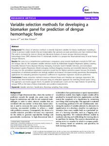
Fig. 1. Surface plot with Cartesian coordinates (c, CR, RX).

the quality of explained variance across the structure and information carried by the full set of original variables. An inspection of surface plot in Fig. 1 shows that an effective use of resources is obtained for a selected subset with six primary variables. VI. CONCLUSION

B. Variable Selection with Pre-Assigned Roles We applied our proposed variable selection methodology with pre-assigned roles to bumper cover manufacturing process. The number of elements in the sets of primary and secondary variables 1 and 2 are 10 and 14 respectively. In this article we used a backward elimination scheme, which at each step eliminates the less informative variable among the primary variables that have not yet been eliminated. The new variable was eliminated by its inability to supply complementary information for the whole set of variables. The subset of relevant variables was selected in a manner that retains, to some extent, the structure and information carried by the full set of original variables, thereby providing a SPC almost as efficient as we were monitoring all original variables. The results showed that efficient monitoring of this process according to criterion RX in (5) could be attained by using only six primary variables. Shewhart control charts of influence functions of eigenvalues for the covariance matrix were used to monitor components of process variability. These influential control charts, accompanied with process logbook gave clear indications for all known assignable causes present in the process. C. Variable Selection with Cost-Utility Analysis To illustrate variable selection with cost-utility analysis we used only the measurements of ten primary variables. The objective of carrying out a cost–utility analysis is to compare one use of resources with other possible uses. Variable subsets for process monitoring were ranked according to CR values in (9). Based on data from the cover bumper process, a surface plot with Cartesian coordinates (c, CR, RX) is displayed in Fig. 1. A subset of relevant variables that retains, to some extent, the structure and information carried by the full set of original variables should have high RX values and low CR and c values. This allows easy comparison across different selected variable subsets, but still requires value judgments to be made about


This article proposes two new methods to select a reduced number of relevant variables for multivariate statistical process control that makes use of engineering, cost and variability evaluation criteria. In the first method a double reduction of dimensionality is applied to select relevant primary variables that represent well the whole set of variables. In the second methodology a cost-utility analysis is proposed to compare different variable subsets that may be used for process monitoring. The objective of carrying out a cost–utility analysis is to compare one use of resources with other possible uses. The subset of relevant variables is selected in a manner that retains, to some extent, the structure and information carried by the full set of original variables. This strategy mitigates the risk that an assignable cause inducing a shift, that lies entirely in the discarded variables, will go undetected. Just like ordinary PCA the solution of the eigenvalue problem in (4) is not scale invariant, and therefore sometimes it is better to apply the above method to standardized data rather than raw data. In such cases the covariance matrices in their formulation are replaced by the corresponding correlation matrices. REFERENCES [1]

[2]

[3]

[4]

[5]

N.M. Al-Kandari, and I.T. Jolliffe, “Variable selection and interpretation of covariance principal components”, Commun. Stat.Simul. Comput, vol. 30, 2001, pp 339-354. N.M. Al-Kandari, and I.T. Jolliffe, “Variable selection and interpretation in correlation principal components”, Environmetrics, vol. 16, 2005, pp 659-672. J.F.C.L. Cadima and I.T. Jolliffe, “Variable selection and the interpretation of principal subspaces”, J. Agric. Biol. Environ. Stat., vol. 6, 2001, pp. 62-79. B. M. Colosimo, Q. Semeraro, and M. Pacella, “Statistical Process Control for Geometric Specifications: On the Monitoring of Roundness Profiles”, Journal of Quality Technology , vol. 40, 2008, pp. 1–18. J. A. Cumming and D. A. Wooff, “Dimension Reduction Via Principal Variables”, Computational Statistics and Data Analysis 52, 2007, pp. 550–565.

WCE 2014

Proceedings of the World Congress on Engineering 2014 Vol II, WCE 2014, July 2 - 4, 2014, London, U.K. [6]

[7]

[8]

[9]

[10]

[11]

[12]

[13] [14] [15] [16] [17] [18]

[19]

I. Gonzalez and I. Sanchez, “Variable Selection for Multivariate Statistical Process Control », Journal of Quality Technology, vol. 42, n°. 3, 2010, pp. 242-259. F.R. Hampel, E.M. Ronchetti, P.J. Rousseew, W.A. Stahel, “Robust Statistics - The Approach Based on Influence Functions”, Wiley, 1986, New-York. W. Krzanowski, “Selection of Variables to Preserve Multivariate Data Structure, Using Principal Components”, Applied Statistics 26, 1987, pp. 22–33. L. Jaupi and G. Saporta, “Using the Influence Function in Robust Principal Components Analysis”. In S. Morgenthaler, E. Ronchetti and W.A. Stahel, eds., New Directions in Statistical Data Analysis and Robustness, Birkhäuser Verlag Basel, 1993, pp. 147-156. L. Jaupi, “Multivariate Control Charts for Complex Processes”. In C. Lauro, J. Antoch, V. Esposito, G. Saporta eds., Multivariate Total Quality Control, Springer, 2001, pp. 125-136. L. Jaupi , D. Herwindiati, P. Durand and D. Ghorbanzadeh, “Short Run Multivariate Control Charts for Process Mean and Variability”, Proc. World Congress on Engineering, 2013, Vol. I, pp.670-674. L. Jaupi , P. Durand , D. Ghorbanzadeh and D. E. Herwindiati, “Multi-Criteria Variable Selection for Process Monitoring”, 59th World Statistical Congress, August 2013. I. T. Jolliffe, “Discarding Variables in a Principal Component Analysis I: Artificial Data”. Applied Statistics 21, 1972, pp. 160–173. I. T. Jolliffe, “Discarding Variables in a Principal Component Analysis II: Real Data”. Applied Statistics 22, 1973, pp. 21–31. I. T. Jolliffe, Principal Components Analysis, 2nd edition. New York, NY: Springer, 2002. G. P. McCabe, “Principal Variables”. Technometrics 26, 1984, pp. 137–144. C.R. RAO, “The Use and Interpretation of Principal Components in Applied Research”. Sankhya, A, 26, 1964, pp. 329-358. Y. Tanaka, and Y. Mori, “Principal component analysis based on a subset of variables: Variable selection and sensitivity analysis”. Amer. J. Mathematical and Management Sciences, 17, 1 & 2, 1997, pp. 61-89. W. H. Woodall, D. J. Spitzner, D. C. Montgomery and S. Gupta, “Using Control Charts to Monitor Process and Product Quality Profiles”. Journal of Quality Technology, vol. 36, 2004, pp. 309– 320.


WCE 2014