r 1999 Wiley-Liss, Inc.
Cytometry 35:162–168 (1999)
Variable Selection and Multivariate Methods for the Identification of Microorganisms by Flow Cytometry Hazel M. Davey,* Alun Jones, Adrian D. Shaw, and Douglas B. Kell Institute of Biological Sciences, University of Wales, Aberystwyth, Ceredigion, Wales, United Kingdom Received 27 January 1998; Revision Received 2 September 1998; Accepted 5 October 1998
Background: When exploited fully, flow cytometry can be used to provide multiparametric data for each cell in the sample of interest. While this makes flow cytometry a powerful technique for discriminating between different cell types, the data can be difficult to interpret. Traditionally, dual-parameter plots are used to visualize flow cytometric data, and for a data set consisting of seven parameters, one should examine 21 of these plots. A more efficient method is to reduce the dimensionality of the data (e.g., using unsupervised methods such as principal components analysis) so that fewer graphs need to be examined, or to use supervised multivariate data analysis methods to give a prediction of the identity of the analyzed particles. Materials and Methods: We collected multiparametric data sets for microbiological samples stained with six cocktails of fluorescent stains. Multivariate data analysis methods were explored as a means of microbial detection and identification.
Results: We show that while all cocktails and all methods gave good accuracy of predictions (G94%), careful selection of both the stains and the analysis method could improve this figure (to G99% accuracy), even in a data set that was not used in the formation of the supervised multivariate calibration model. Conclusions: Flow cytometry provides a rapid method of obtaining multiparametric data for distinguishing between microorganisms. Multivariate data analysis methods have an important role to play in extracting the information from the data obtained. Artificial neural networks proved to be the most suitable method of data analysis. Cytometry 35:162–168, 1999. r 1999 Wiley-Liss, Inc.
Flow cytometry (1) is a rapid method for the analysis of single cells as they flow in a liquid medium through the focus of a laser beam surrounded by an array of detectors. When exploited fully, flow cytometry yields a multiparametric set of measurements relating to each cell that is analyzed. These measurements may be of intrinsic cell properties such as forward light scattering, which provides a measure of cell size (2–4), side scattering, which gives a measure of granularity, or autofluorescence. Alternatively, the investigator may add one or more fluorescent stains to the sample prior to analysis, allowing the measurement of a variety of determinands (5,6). Many different fluorescent stains, with a variety of cellular targets, have been investigated by flow cytometry. These include stains that have a high specificity for nucleic acids, proteins, or lipids, and probes which reflect Ca2⫹ concentration, pHin, etc. (4,7,8). When selecting a combination of fluorescent stains to use together in a cocktail, there are several factors that need to be considered. These include the facts that 1) the stains must be excited efficiently by the light sources available, 2) the emission wavelengths should not overlap (although if they are excited by different light sources their
emissions can be separated by gated-amp electronics), and 3) the cellular targets of the constituents of the cocktails should be different. Flow cytometry enables the experimenter to analyze large numbers of cells at high speeds (1,9,10). With typical rates of data acquisition being on the order of 100–1,000 cells.s⫺1 (thus enabling the collection of data from tens of thousands of cells per sample rather quickly), large amounts of data are produced. Flow cytometric data are collected in many prototype or commercial instruments that reflect 3–8 (11,12) or even more (13–15) different parameters, such that sophisticated data processing techniques are desirable in order to extract the most useful information from the data (5,16–18). Principal components analysis (PCA) (19,20) is a useful aid in the visualization of multivariate data. The aim of PCA
Key terms: artificial neural networks; microorganism; multivariate data analysis; principal components; variable selection
Contract grant sponsor: European Research Office of the United States Army; Contract grant sponsor: BBSRC/LINK; Contract grant sponsor: Higher Education Funding Council for Wales. *Correspondence to: Hazel M. Davey, Institute of Biological Sciences, University of Wales, Aberystwyth, Ceredigion SY23 3DD, Wales, UK. E-mail:
[email protected]
MULTIVARIATE DATA ANALYSIS METHODS
is to rotate the data points into a new coordinate system, such that the majority of the variance in the data set is accounted for in the directions of a subset of these rotated axes. Hence, by plotting the points in this new coordinate system, the significant effects within the data can be more easily visualized. PCA is an ‘‘unsupervised’’ method, in that it examines only the measured variables in order to perform the analysis, and does not take the class structure of the data into account. Hence, PCA can (and is likely to) highlight effects that are not of direct interest to the experiment at hand. Unsupervised methods are ideal for a preliminary examination of the data (21), but do not directly aid in the formation of predictive models. For this application, one is forced to use the more sophisticated ‘‘supervised’’ methods such as principal components regression (PCR), partial least squares regression (PLSR) (22), and artificial neural networks (ANNs) (23–27). PCR is a simple extension of PCA, in that a multiple linear regression (MLR) is performed on a subset of the values of the principal components. If the first few components do indeed reflect relevant variations, PCR can give rise to a useful model, where MLR would fail due to collinearity. PLSR is a more useful supervised method, as it is designed to extract those underlying linear effects which are of most relevance to the Y data of interest (in this case the identity of the microorganisms). PCR and PLSR are limited, in that they can only take account of linear relationships within the data. If the relationships are suspected to be nonlinear, then ANNs are needed, as these can represent arbitrary (continuously differentiable) nonlinear functions (28). When using multiple variables as inputs to any multivariate analysis, some variables will be found more important than others. Indeed, it often happens that some variables are detrimental to the multivariate calibration model (29). This could be because they are measuring something other than the searched-for correlation, or simply because the information contained is also contained in other variables. The parsimony principle (30) states that where two models give the same result, the simpler model should be preferred, as it will be able better to predict an unseen data set. Therefore, variables which do not contain any additional information are undesirable (31). For this reason, a suite of Microsoft Excel macros has been written to carry out variable selection, with a view to establishing the best variables from which to form a model (32). The majority of flow cytometric research that has been published to date has involved the study of mammalian cells, although numerous areas of microbial research would benefit greatly from the flow cytometric approach (5). One common problem for the microbiologist is the identification of cells within a given sample. This may be, for example, when one is monitoring the progress of an industrial fermentation, where the emphasis may be on the detection of contaminants (33,34), or on the analysis of the physiological changes occurring therein (35–38). Alternatively, it may be that environmental samples are being analyzed for the presence of pathogenic organisms when the release of a biowarfare agent (where the most
163
credible threat is Bacillus anthracis (39,40)) is suspected (41–45). As the flow cytometric approach involves the study of individual cells, it is readily amenable to the problem of identifying specific cell types against a background of other biological and nonbiological particulates. We therefore present a study of a variety of data analysis methods for the analysis of microbial cells, with emphasis on selection of the most appropriate stain cocktail and data analysis method for the detection and identification of Bacillus globigii spores (as a nonpathogenic model for B. anthracis) against a background of other microorganisms. MATERIALS AND METHODS Sample Preparation Bacillus subtilis var niger (B. globigii) spores were obtained from the Chemical and Biological Defence Establishment (CBDE), (Porton Down, Salisbury, UK) as a dry preparation. Prior to analysis the spores were suspended in sheath fluid (see below) to give a concentration of approximately 1 ⫻ 106 spores.ml⫺1. Escherichia coli (Lab Strain C500) were grown on a medium containing 1% tryptone, 1% yeast extract, and 70 mg.1⫺1 MgSO4. The medium was adjusted to pH 6.8 with HCl or KOH prior to autoclaving at 121°C for 15 min. Cells were grown in batch culture at a temperature of 37°C on a shaker for 3 days. Micrococcus luteus (NCIMB 13267) were grown on E-Broth (Lab M) on a shaker at 30°C for 3 days. A strain of Saccharomyces cerevisiae was isolated from locally obtained baker’s yeast, and grown on yeast extract peptone glucose (YPG) medium which contained 5% glucose, 0.5% yeast extract, and 0.5% bacteriological peptone. The medium was adjusted to pH 5 with phosphoric acid prior to autoclaving. Temperature was maintained at 30°C, but the culture flask was not agitated during the 3-day incubation. Fixed cells or spores were prepared by squirting a suspension of spores or cells from a syringe into ethanol to give a final ethanol concentration of 70%. Fixed samples could be stored at ⫺20°C for several months without noticeable deterioration. All fixed samples were centrifuged and washed in the sheath fluid used for flow cytometric analysis (see below) prior to resuspension in sheath fluid. Fixed samples were analyzed within 2 h of removal of the fixative. Fluorescent Stains Tinopal CBS-X (5,46) was obtained as a gift from Ciba Dyes and Chemicals, Ltd. (Macclesfield, UK). Nile red, propidium iodide, and fluorescein isothiocyanate (FITC) were obtained from Sigma (Poole, Dorset, UK). DISC2(5), Oxonol V, SYTO 17, and TO-PRO-3 were obtained from Molecular Probes Europe BV, (Leiden, The Netherlands). These stains were added to the fixed microbial samples in the following order, combination, and concentrations: 1. Tinopal cocktail: Tinopal CBS-X at 40 µg.ml⫺1, propidium iodide at 50 µg.ml⫺1, and FITC at 25 µg.ml⫺1.
DAVEY ET AL.
164
2. Nile red cocktail: Nile red at 10 µg/ml⫺1, propidium iodide at 50 µg.ml⫺1, and FITC at 25 µg.ml⫺1. 3. DiSC2(5) cocktail: Tinopal CBS-X at 40 µg.ml⫺1, DISC2(5) at 1 µg.ml⫺1, and FITC at 25 µg.ml⫺1. 4. Oxonol cocktail: Tinopal CBS-X at 40 µg.ml⫺1, Oxonol V at 1 µg.ml⫺1, and FITC at 25 µg.ml⫺1. 5. SYTO17 cocktail: Tinopal CBS-X at 40 µg.ml⫺1, SYTO 17 at 1 µM (⬃0.65 µg.ml⫺1), and FITC at 25 µg.ml⫺1. 6. TO-PRO-3 cocktail: Tinopal CBS-X at 40 µg.ml⫺1, TO-PRO-3 at 1 µM (0.67 µg.ml⫺1), and FITC at 25 µg.ml⫺1. Flow Cytometry All flow cytometric analyses were performed using a Coulter Epics Elite flow cytometer (Coulter Electronics, Ltd., Luton, UK) equipped with the following three lasers which were suitable for excitation of all of the stains used in this study. The numbers in parentheses show the laser wavelengths used and the emission wavelengths that were collected for each stain: Helium-cadmium laser (325 nm) Tinopal CBS-X (⬍440 nm and 525 nm) Argon ion laser (488 nm) FITC (525 nm) Nile red (575 nm) Propidium iodide (⬎600 nm) Helium-neon laser (633 nm) DISC2(5) (675 nm) Oxonol V (675 nm) SYTO 17 (675 nm) TO-PRO-3 (675 nm). In addition, forward scatter, side scatter, and where appropriate, autofluorescence (575 nm) signals were collected from the argon ion laser. The flow cytometer was set up as described in the manufacturer’s manual, and a logarithmic gain was used in all cases. The sheath fluid was prepared using Millipore Milli-Q water filtered to 0.2 µm and contained 150 mM KCl and 10 mM HEPES. The sheath fluid was adjusted to pH 6.8 with KOH and then filtered using a 0.1-µm Whatman WCN filter. Prepared sheath fluid was stored at 4°C but was allowed to reach room temperature before use. The lasers were aligned (using Coulter Immunocheck beads) so that the sample intersected the HeCd laser 40 µs after intersecting the argon ion and HeNe lasers. The signals were then recombined using the gated amp electronics. Thus, cocktails were created that consisted of dyes with separable fluorescence characteristics and different cellular targets. Nucleic acids were, in the various cocktails, stained by either propidium iodide, SYTO-17, or TOPRO-3. FITC labels protein, and Nile red binds preferentially to lipids. The exact targets of the other dyes used were not completely clear in the case of vegetative or sporulated bacteria (e.g., see Davey and Kell (46)), but for the present work it is the multidimensional pattern of staining rather than the physiological interpretation of the staining that is important.
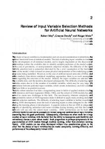
FIG. 1. Schematic representation of the data analysis protocol. For a given stain cocktail, the list-mode files for each of the microorganisms were converted to ASCII format, using the lldata utility (for more information see the online catalogue of free flow cytometry software http://www.bio.umass.edu/mcbfacs/flowcat.html). Subset.bas was written in-house using Microsoftt Qbasic (and is available from http:// pcfcij.dbs.aber.ac.uk/software.htm) to select every nth, event from the data file to give a user-defined number of events. Partial least squares (PLSR), principal components regression (PCR), and artificial neural networks (ANNs) were then performed from within the Microsoftt Excel spreadsheet, using macros that interfaced to executable C code, both of which were written in-house.
Data Analysis Data sets containing representatives of each of the four organisms studied were created by combining events from separate list-mode files, as shown in Figure 1. Ideally, one may wish to use samples that were mixed prior to flow
MULTIVARIATE DATA ANALYSIS METHODS
165
Table 1 Summary of Results of Multivariate Data Analysis of Flow Cytometric Data for Six Cocktails used to Identify Those Events that Correspond to Bacillus globigii in the Data Set
Comment or data analysis method Instrument complexitya Data complexityb Variable rankingc
Raw plot of best variablesd PCAd PLSRe
PCRe
ANNf Epochsg Thresholdh
Nile Red PI FITC 1 laser
Tinopal PI FITC 2 lasers
Cocktail of fluorescent dyes Tinopal Tinopal DiSC2(5) Oxonol V FITC FITC 3 lasers 3 lasers
5 variables PI Nile Red FS FITC Side scatter
7 variables Autofluor. PI FS FITC Side scatter Tinopal 440 Tinopal 525 PI/FS %B 98% %notB 99.5 Factors 1 & 3 %B 98.5 %notB 96.8 Best were 5, 6, or 7 variables %B 100 %notB 99 Best were 5, 6, or 7 variables %B 100 %notB 99 7-3-1 10,000 0.37–0.57 %B 100 %notB 99.3
7 variables FITC FS Tinopal 440 Side scatter Autofluor. Tinopal 525 DiSC2(5) FITC/FS %B 99.5 %notB 98.8 Factors 1 & 2 %B 99 %notB 95.8 Best was 7 variables %B 98 %notB 100 Best were 6/7 variables %B 99 %notB 99.3 7-3-1 1,000,000 0.49–0.5 %B 100 %notB 100
PI/FS %B 99 %notB 98.3 Factors 1 & 2 %B 100 %notB 99 Best was 5 variables %B 100 %notB 98 Best was 5 variables %B 100 %notB 98 5-3-1 11,000 0.5–0.62 %B 100 %notB 99
7 variables FITC Oxonol FS Tinopal 440 Autofluor. Side scatter Tinopal 525 FITC/FS %B 100 %notB 95.8 Factors 1 & 2 %B 99.5 %notB 94.8 Best was 7 variables %B 100 %notB 96.7 Best was 7 variables %B 100 %notB 96.7 7-3-1 10,000 0.56 %B 99 %notB 97.7
Tinopal SYTO 17 FITC 3 lasers
Tinopal TOPRO-3 FITC 3 lasers
7 variables FITC FS Tinopal 440 Side scatter Autofluor. SYTO 17 Tinopal 525 FITC/FS %B 100 %notB 97.5 Factors 1 & 2 %B 98.5 %notB 96.3 Best was 7 variables %B 100 %notB 95.7 Best was 7 variables %B 100 %notB 95.7 7-3-1 1,000,000 0.76–0.77 %B 100 %notB 99
7 variables TO-PRO-3 FITC FS Autofluor. Tinopal 440 Side scatter Tinopal 525 FITC/FS %B 100 %notB 97.8 Factors 1 & 2 %B 100 %notB 96.2 Best was 7 variables %B 100 %notB 97 Best was 3 variables %B 99 %notB 96.3 7-3-1 100,000 0.54–0.59 %B 100 others 99
Grey-shaded squares indicate that, by using a given cocktail/data analysis method combination, 99%⫹ of the events were correctly identified. PI, propidium iodide; FS, forward scatter; FITC, fluorescein isothiocyanate; Autofluor., autofluorescence at 575 nm; %B, percentage of Bacillus globigii spores correctly identified; %notB, percentage of non-Bacillus globigii events that were correctly identified. aThree dyes were used in each cocktail, but the complexity of the instrument required to analyze the samples varied. The Nile red/PI/FITC combination is an example of a cocktail where all of the dyes can be excited by a single laser. In certain circumstances a single laser instrument may be preferrable for reasons of expense and ease of operation. bDifferent cocktails yielded different amounts of data about the cells being analyzed. The more variables collected, the easier it should be to discriminate between various particle types present in the sample. However, a larger number of variables makes traditional data analysis methods more difficult. cThe Fisher method was used to rank the variables, and they are shown here with the most discriminatory variable at the top of the list. dIn the case of the raw data and the PCA, the ‘‘best’’ graph was determined by eye from the combinations of the best three (Fisher-selected) variables. Regions were drawn that best separated the Bacillus globigii events from the other organisms, i.e., gave the fewest false positives and false negatives. The best raw graph is indicated here by the two variables chosen; the best PCA graph is indicated by the two factors that were chosen. eThe PLSR and PCR analyses were carried out as described in the text. In most but not all cases, the analysis that used all of the variables gave the best results, indicating that there was no redundancy in the data. fA standard back-propagation neural network was used in all cases. The architecture of the network used was as shown here, e.g., 5-3-1 indicates that there were 5 nodes in the input layer (corresponding to the 5 variables in the data set which were normalized between 0.2–0.8), 3 nodes in the hidden layer, and 1 node in the output layer. gThe number of epochs required to produce an optimally trained network (as judged by counting the number of errors in the test set) is indicated. The larger the number of epochs, the longer it will take to produce the trained network. However, once the model is produced, the interrogation time for all networks is the same, and is very fast (1–2 s using a Pentium 200 with the 400 element test sets used here). hThe threshold for the neural network prediction is the ‘‘line’’ drawn between positive and negative events. The networks were trained to give a 1 for Bacillus globigii and a 0 for all other particle types. A broad threshold range (such as that obtained with the Tinopal cocktail) indicates that the predictions are well-separated, and thus the model should be more robust.
cytometric analysis to create and test the models, but in this case there would be no a priori knowledge of the identity of the individual events in the list-mode file to test the accuracy of the models. However, we studied the dual-parameter histograms produced from preacquisition
mixtures and postacquisition mixtures and found no differences that would indicate modulation of fluorescence intensity or interspecies clumping. Furthermore, using a trained ANN to predict the identity of 5,000 unknown events from the analysis of a preacquisition
166
DAVEY ET AL.
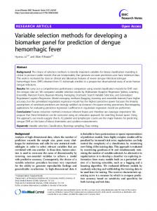
FIG. 2. FITC (protein) fluorescence and forward light scattering were the two most discriminatory variables obtained from analysis of samples stained with the SYTO 17 cocktail. The data (plotted as channel numbers) were collected using the Coulter Epics Elite flow cytometer, as described in Materials and Methods. Two hundred events for each organism were plotted. The voltage for the forward scatter detector was set to 400, and a voltage of 570 was used for the FITC signal. In both cases the gain was logarithmic. A polygon was drawn around the Bacillus globigii data (squares). There were no false negatives (squares outside the polygon), but there were 15 (2.5%) false positives (other symbols within the polygon). Triangles represent E. coli, circles represent M. luteus, and diamonds represent yeast cells.
mixture resulted in a prediction of 19.8% B. globigii compared to the 19% that would have been expected from counting. The data were analyzed with a variety of multivariate methods according to the protocol shown in Figure 1. The method of selecting the variables is called CalcW (32): this calculates a value referred to as w, which represents how good each variable is for classification. The lower the value of w, the better the variable. Initially, a model is formed using all the variables and then, using w as a guide, one variable at a time is deleted and a new model formed. In this way, the best number of variables can be found. For sets of data with a large number of variables, this number is invariably much lower than the total number of variables. For sets of data of the size presented here, variable selection is of lesser use, but nonetheless is worthwhile to ensure that models use the optimum number of variables. Where an accurate result can be obtained with a smaller number of variables, this is to be preferred, as the resulting model will be simpler and the sample preparation and data collection system can also be simplified. It should be noted that not all combinations of variables have been tried; rather, judicious selection is used to attempt to find the optimum variables. The reason for this is that with larger numbers of variables, it is not practical to try all combinations. RESULTS AND DISCUSSION The most common method of analysis for flow cytometric data is to study combinations of single- or dualparameter histograms for each of the samples analyzed. As the number of measured parameters (n) increases, the number of dual-parameter plots that need to be inspected if one is to examine each possible dual-parameter plot increases as n(n ⫺ 1)/2. In the examples presented here, 5 or 7 parameters were collected, depending on the cocktail used (see Table 1). Thus, a full exploration of the data would involve the inspection of 10 or 21 plots, respectively. Thus, we used a variable selection method based on the Fisher ratio (32) (hence referred to as the Fisher method), which is essentially the ratio of within-group variance to between-group variance (30,32) to select the
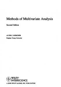
most discriminatory variables from the 5 or 7 available, and we plotted the best three in each two-dimensional (2D) combination to determine what degree of separation can be achieved (e.g., see Fig. 2). In the case of the SYTO 17 cocktail shown in Figure 2, a line can be drawn to define a region on the 2D plot of the most discriminatory variables that contains all of the Bacillus globigii events (200) that were included in the data set. However, there are also some E. coli and M. luteus within the region (false positives). This process was repeated for each of the cocktails, and the best results for each cocktail were recorded in Table 1. In the current work, variable selection was used as a method of choosing the most discriminatory variables (flow cytometric parameters) for producing a small number of dual-parameter plots from a multiparametric data set. However, since the Fisher ratio ranks the variables according to their ability to discriminate between the particles of interest, the method could also be used for optimizing combinations of dyes to produce the most discriminatory cocktail. The second method that was investigated was PCA. Again, one is looking for clustering of the B. globigii events at a discrete location from those of the other organisms (e.g., see Fig. 3). PCA should allow for a better separation of the clusters than simply plotting the raw data, because the variance of the data set is preserved in a smaller number of factors. However, with 5 out of the 6 cocktails in the present study, the opposite was found to be true (see Table 1), with PCA giving worse predictions than simply plotting the raw data, despite the fact that the first component accounted for between 69.7–80.2% of the variance (not shown). The reason for this is that PCA will extract as its primary factors the dimensions of greatest variance. It does not necessarily follow that the first few components are characteristic of the substance under analysis; they could well be due to some other factor. This is one of the major pitfalls of using ‘‘unsupervised’’ methods such as PCA. In comparison, the other methods used (PLSR, PCR, and ANNs) are all ‘‘supervised’’ methods. With supervised methods it is necessary to split the data set into a training
MULTIVARIATE DATA ANALYSIS METHODS
167
FIG. 3. The two most discriminatory PCA factors from the analysis of the SYTO 17 cocktail were plotted. Two hundred events for each organism were plotted. A line was drawn to separate the Bacillus globigii data (squares) from the other data. There were 3 false negatives (1.5%) and 22 false positives (3.7%). Symbols for the other organisms are as shown in the legend to Figure 2.
set and at least one test set. The training set is then used to form the model, and the test sets are used to assess how well the model performs. PLSR and PCR were first performed with all available variables. The least discriminatory of these was then deleted from the data set, and a new model was made. This was continued until only one variable remained. Each of the models so formed was assessed with the appropriate test set, and the accuracy of the prediction with the optimal number of variables was recorded in Table 1. In the case of ANNs, the creation of a useful model (training process) was more time-consuming. Consequently they were used only with the full data sets, using a 5-3-1 (Fig. 4A) or 7-3-1 architecture depending on the number of measured parameters. The training process involved repeated presentations of the training set (measured inputs and expected output) to the network. Internal weights associated with the connections between the layers (Fig. 4A) were adjusted to reduce the error between the expected output and the predicted output. Each complete presentation of the training set is referred to as an epoch. The training process was stopped at various points, and the nets were tested with the test set (Fig. 4B). The optimally trained ANN was selected for each of the cocktails, and the predictions were recorded in Table 1. One of the problems associated with the flow cytometric analysis of microorganisms is that microbes tend to form clumps. Flow cytometers make measurements on individual particles, but because of the size variability of microbial cells, it is often difficult or impossible to determine whether a given particle consists of a single cell or a clump of two or more cells. However, provided that enough examples of clumped cells are included in the training set, supervised methods may be expected to identify these particles correctly. Table 1 confirms that this is the case, since good predictions (95.7%⫹) were obtained with all cocktails and all supervised data analysis methods. However, the best results were obtained with
FIG. 4. A: Example of a fully interconnected back-propagation neural network with a 5-3-1 architecture. There are 5 nodes in the input layer, each representing one of the measured parameters. The input nodes are connected to the three nodes in the hidden layer, and the hidden layer is connected to the output layer. During the training process, the ANN was presented with a series of data patterns on the input layer, each pattern representing one of the four organisms that were analyzed, together with a corresponding output (all of these values were scaled between 0.2–0.8 before presentation to the network). The network was taught to predict a value close to 1 if the pattern represented B. globiggi, and a value close to 0 if any other organism was presented. B: Example of the predicton of a test set by an optimally trained neural network. The grey-shaded area (threshold; see Table 1) separates the positive and negative predictions. Misidentifications were noted, along with the results for the other cocktails, in Table 1.
DAVEY ET AL.
168
the Tinopal cocktail, where all supervised methods gave 99%⫹ accuracy. The best overall data analysis method was the artificial neural network approach where, with the exception of the Oxonol cocktail, 99%⫹ accuracy was achieved in all cases. In conclusion, flow cytometry is a valuable technique for the detection of spores against a background of other microorganisms. By the careful selection of an appropriate staining cocktail and a suitable data analysis method, very accurate identifications can be made. ACKNOWLEDGMENTS We thank Ciba Dyes and Chemicals, Ltd., for the gift of Tinopal CBS-X. H.M.D. and D.B.K. were supported by the European Research Office of the U.S. Army. A.D.S. was supported by BBSRC/LINK. A.J. was supported by the Higher Education Funding Council for Wales. LITERATURE CITED 1. Shapiro HM. Practical flow cytometry, 3rd ed. New York: Alan R. Liss, Inc.; 1995. 2. Davey HM, Davey CL, Kell DB. On the determination of the size of microbial cells using flow cytometry. In: Lloyd D, editor. Flow cytometry in microbiology. London: Springer-Verlag; 1993. p 49–65. 3. Koch AL, Robertson BR, Button DK. Deduction of the cell volume and mass from forward scatter intensity of bacteria analyzed by flow cytometry. J Microbiol Methods 1996;27:49–61. 4. Salzman GC, Singham SB, Johnston RG, Bohren CF. Light scattering and cytometry. In: Melamed MR, Lindmo T, Mendelsohn ML, editors. Flow cytometry and sorting, 2nd ed. New York: Wiley-Liss, Inc.; 1990. p 81–107. 5. Davey HM, Kell DB. Flow cytometry and cell sorting of heterogeneous microbial populations: the importance of single-cell analyses. Microbiol Rev 1996;60:641–696. 6. Waggoner AS. Fluorescent probes for cytometry. In: Melamed MR, Lindmo T, Mendelsohn ML, editors. Flow cytometry and sorting, 2nd ed. New York: Wiley-Liss Inc.; 1990. p 209–225. 7. Grogan WM, Collins JM. Guide to flow cytometry methods. New York: Marcel Decker, Inc.; 1990. 8. Haugland RP. Molecular Probes handbook of fluorescent probes and research chemicals, 6th ed. Molecular Probes, Inc.; 1996. 9. Lloyd D. Flow cytometry: a technique waiting for microbiologists. In: Lloyd D, editor. Flow cytometry in microbiology. London: SpringerVerlag; 1993. p 1–9. 10. Melamed MR, Lindmo T, Mendelsohn ML. Flow cytometry and sorting, 2nd ed. New York: Wiley-Liss, Inc.; 1990. 11. Kachel V, Messeschmidt R, Hummel P. Eight-parameter PC-AT based flow cytometric data system. Cytometry 1990;11:805–812. 12. Steinkamp JA, Habbersett RC, Hiebert RD. Improved multilaser/ multiparameter flow cytometer for analysis and sorting of cells and particles. Rev Sci Instrum 1991;62:2751–2764. 13. Dubelaar GBJ, Groenewegen AC, Stokdijk W, van den Engh GJ, Visser JWM. Optical plankton analyzer—a flow cytometer for plankton analysis. 2. Specifications. Cytometry 1989;10:529–539. 14. Peeters JCH, Dubelaar GBJ, Ringelberg J, Visser JWM. Optical plankton analyzer—a flow cytometer for plankton analysis. 1. Design considerations. Cytometry 1989;10:522–528. 15. Robinson JP, Durack G, Kelley S. An innovation in flow cytometry data collection and analysis producing a correlated multiple sample analysis in a single file. Cytometry 1991;12:82–90. 16. Boddy L, Morris CW. Neural network analysis of flow cytometry data. In: Lloyd D, editor. Flow cytometry in microbiology. London: SpringerVerlag; 1993. p 159–169. 17. Givan AL. Flow cytometry first principles. New York: Wiley-Liss, Inc.; 1992. 18. Watson JV. Flow cytometry data analysis: basic concepts and statistics. Cambridge: Cambridge University Press; 1992.
19. Hotelling H. Analysis of a complex of statistical variables into principal components. J Educ Psychol 1933;24:417–441, 498–520. 20. Jolliffe IT. Principal component analysis. Heidelberg: Springer; 1986. 21. Tukey JW. Exploratory data analysis. Reading, MA: Addison-Wesley; 1977. 22. Martens H, Næs T. Multivariate calibration. Chichester: John Wiley; 1989. 23. Balfoort HW, Snoek J, Smits JRM, Breedveld LW, Hofstraat JW, Ringelberg J. Automatic identification of algae: neural network analysis of flow cytometric data. J Plankton Res 1992;14:575–589. 24. Boddy L, Morris CW. Analysis of flow cytometry data—a neural network approach. Binary 1993;5:17–22. 25. Frankel DS, Olson RJ, Frankel SL, Chisholm SW. Use of a neural net computer system for analysis of flow cytometric data of phytoplankton populations. Cytometry 1989;10:540–550. 26. Morris CW, Boddy L, Allman R. Identification of Basidiomycete spores by neural network analysis of flow cytometry data. Mycol Res 1992;96:697–701. 27. Næs T, Kvaal K, Isaksson T, Miller C. Artificial neural networks in multivariate calibration. J Near Infrared Spec 1993;1:1–11. 28. White H. Artificial neural networks: approximation and learning theory. Oxford: Blackwell; 1992. 29. Kell DB, Sonnleitner B. GMP—good modelling practice. Trends Biotechnol 1995;13:481–492. 30. Seasholtz MB, Kowalski B. The parsimony principle applied to multivariate calibration. Anal Chim Acta 1993;277:165–177. 31. Miller AJ. Subset selection in regression. London: Chapman & Hall; 1990. 32. Shaw AD, di Camillo A, Vlahov G, Jones A, Bianchi G, Rowland J, Kell DB. Discrimination of the variety and region of origin of extra virgin olive oils using 13C NMR and multivariate calibration with variable reduction. Anal Chim Acta 1997;348:357–374. 33. Jespersen L, Lassen S, Jakobsen M. Flow cytometric detection of wild yeast in lager breweries. Int J Food Microbiol 1993;17:321–328. 34. Urano N, Nomura M, Sahara H, Koshino S. The use of flow cytometry and small-scale brewing in protoplast fusion—exclusion of undesired phenotypes in yeasts. Enzyme Microbial Technol 1994;16:839–843. 35. Alberghina L, Ranzi BM, Porro D, Martegani E. Flow cytometry and cell cycle kinetics in continuous and fed-batch fermentations of budding yeast. Biotechnol Prog 1991;7:299–304. 36. Davey HM, Davey CL, Woodward AM, Edmonds AN, Lee AW, Kell DB. Oscillatory, stochastic and chaotic growth rate fluctuations in permittistatically-controlled yeast cultures. Biosystems 1996;39:43–61. 37. Dinsdale MG, Lloyd D, Jarvis B. Yeast vitality during cider fermentation—2 approaches to the measurement of membrane-potential. J Institute Brewing. 1995;101:453–458. 38. Scheper T, Gebauer A, Sauerbrei A, Niehoff A, Schugerl K. Measurement of biological parameters during fermentation processes. Anal Chim Acta 1984;163:111–118. 39. Dando M. Biological warfare in the 21st century. London: Brassey’s; 1994. 40. Rimmington A. Russia’s military microbiologists record victory against anthrax, but at what civillian cost? Microbiol Eur 1994;2:12–13. 41. Davey HM, Kell DB. Rapid flow cytometric detection and identification of microbial particles using multiple stains and neural networks. Presented at the Scientific Conference on Chemical and Biological Defense Research, 1996, Edgewood, Baltimore, MD. ERDEC-SP-048. Baltimore: Aberdeen Proving Ground; 1997. p 393–399. 42. Davey HM, Kell DB. A portable flow cytometer for the detection and identification of microorganisms. In: Proceedings of the NATO Advanced Research Workshop on Rapid Methods for Monitoring the Environment for Biological Hazards. Warsaw, Poland: in press. 43. Phillips AP, Martin KL. Immunofluorescence analysis of Bacillus spores and vegetative cells by flow cytometry. Cytometry 1983;4:123– 131. 44. Phillips AP, Martin KL. Dual-parameter scatter-flow immunofluorescence analysis of Bacillus spores. Cytometry 1985;6:124–129. 45. Phillips AP, Martin KL, Broster MG. Differentiation between spores of Bacillus anthracis and Bacillus cereus by a quantitative immunofluorescence technique. J Clin Microbiol 1983;17:41–47. 46. Davey HM, Kell DB. Fluorescent brighteners: novel stains for the flow cytometric analysis of microorganisms. Cytometry 1997;28:311–315.