Variance Reduction in the Simulation of Call Centers

Proceedings of the 2006 Winter Simulation Conference L. F. Perrone, F. P. Wieland, J. Liu, B. G. Lawson, D. M. Nicol, and R. M. Fujimoto, eds.

VARIANCE REDUCTION IN THE SIMULATION OF CALL CENTERS

Pierre L’Ecuyer Eric Buist D´epartement d’Informatique et de Recherche Op´erationnelle Universit´e de Montr´eal, C.P. 6128, Succ. Centre-Ville Montr´eal (Qu´ebec), H3C 3J7, CANADA

ABSTRACT We show via concrete illustrations how the variance can be reduced in the simulation of a telephone call center to estimate the fraction of calls answered within a given time limit. We examine the combination of a control variate and stratification with respect to a continuous input variable, and find that combining them requires care, because the optimal control variate coefficient is a function of the variable on which we stratify. In a setting where we compare two similar configurations of the center, we examine the combination of stratification with common random numbers. We show that proper use of common random numbers reduces the convergence rate of the variance of the difference of performance measures across the two systems.

variate (CV) for this model. The stratification is with respect to a uniform random number that drives the simulation. The optimal CV coefficient depends on the realization of this uniform and there is also an interdependence between the CV coefficients and the optimal allocation in strata. This type of combination is non-standard and requires some care. In Section 4, we study the efficiency of using common random numbers to estimate the sensitivity with respect to a parameter of the service time distribution. This is nontrivial mainly because the sample performance is discontinuous with respect to this parameter. Most examples are adapted from the future book of L’Ecuyer (2006). The simulations were all made with ContactCenters, a specialized simulation tool for contact centers (Buist and L’Ecuyer 2005) developed in Java with the SSJ library (L’Ecuyer and Buist 2005).

1

2

INTRODUCTION

Telephone call centers, and more generally contact centers where mail, fax, e-mail, and Internet contacts are handled in addition to telephone calls, are important components of large organizations (Gans, Koole, and Mandelbaum 2003). One of the main problems in managing these centers is to optimize the number of agents who talk with customers over the phone, and the working schedules of these agents, under constraints on the quality of service and on admissible schedules. Large call centers are complex stochastic systems that can be analyzed realistically only by simulation; tractable queueing models oversimplify reality and are not very reliable. When simulation is combined with an optimization algorithm, its efficiency is a key issue, because optimization often requires thousands of simulation runs at different parameter settings (Cez¸ik and L’Ecuyer 2006). In this paper, we take a simulation model of a (simplified) call center inspired from real life and we experiment with different ways of reducing the variance without significantly increasing the computing cost. The basic model is described in Section 2. In Section 3, we study the combination of stratification with a control

1-4244-0501-7/06/$20.00 ©2006 IEEE

A SMALL MODEL OF A CALL CENTER

We consider a (simple) model of a telephone call center where agents answer incoming calls. Real-life call centers often have separate groups of agents having different combinations of skills that enable them to handle only a subset of the different types of calls. Here, to simplify the presentation, we assume a single type of agent and a single type of call. Otherwise, the model is strongly inspired by a real-life center in Canada. The techniques that we discuss also apply to more complex centers and other similar types of queueing systems. Each day, the center operates for m hours. The number of agents answering calls and the arrival rate of calls vary during the day; we shall assume that they are constant within each hour of operation but depend on the hour. Let n j be the number of agents in the center during hour j, for j = 0, . . . , m − 1. For example, if the center operates from 8 AM to 9 PM, then m = 13 and hour j starts at ( j + 8) o’clock. All agents are assumed identical. If more than n j+1 agents are busy at the end of hour j, calls in progress are completed but new calls are answered only when there are fewer than n j+1 agents busy. After the center closes,

604

L’Ecuyer and Buist We ran a simulation experiment with n = 10000. The sample mean and sample variance of the Xi ’s were X¯n = 1418.0 and Sn2 = 77418, respectively. The estimated variance of X¯n is thus 7.74. Next, we show how to reduce this variance.

ongoing calls are completed and calls already in the queue are answered, but no additional incoming call is taken. The calls arrive according to a Poisson process with piecewise constant rate, equal to R j = Bλ j during hour j, where the λ j are constants and B is a random variable with mean 1 that represents the busyness factor of the day. We suppose that B has the gamma distribution with parameters (α0 , α0 ), i.e., with mean E[B] = 1 and Var[B] = 1/α0 . The Poisson process assumption means that conditional on B, the number of incoming calls during any subinterval (t1 ,t2 ] of hour j is a Poisson random variable with mean (t2 −t1 )R j and that the arrival counts in any disjoint time intervals are independent. This type of arrival process model is motivated and studied by Whitt (1999) and Avramidis, Deslauriers, and L’Ecuyer (2004). Incoming calls form a FIFO queue for the agents. A call abandons (and is lost) when its waiting time exceeds its patience time. The patience times of calls are assumed to be i.i.d. random variables with the following distribution: with probability p the patience time is 0 (so the person hangs up if no agent is available immediately), and with probability 1 − p it is exponential with mean 1/ν. The service times are i.i.d. gamma random variables with parameters (α, γ), i.e., with mean α/γ and variance α/γ 2 . We want to estimate g(s0 ), the fraction of calls whose waiting time is less than s0 seconds (including those who abandoned before s0 seconds), for a given threshold s0 , over infinite time horizon (i.e., an infinite number of days). This g(s0 ) is called the service level and is by far the most widely used measure of quality of service in call centers. In many cases, it is even regulated by law. Let A be the number of arriving calls during the day and X = G(s0 ) the number of those calls waiting less than s0 seconds. The expected number of arrivals is a = E[A] = ∑m−1 j=0 λ j and we have g(s0 ) = E[G(s0 )]/a. Since a is known, here we will estimate µ = a · g(s0 ) = E[G(s0 )]. We simulate the model for n days. For each day i, let Ai be the number of arrivals and Xi = Gi (s0 ) the number of calls who waited less than s0 seconds. A straightforward (or crude) unbiased estimator of µ is

3

COMBINING STRATIFICATION WITH A CONTROL VARIATE

3.1 Stratification on B Noting that the value of B is obviously an important source of variance for X = G(s0 ), a first idea would be to stratify on B. We can partition the set of all possible values of B in k strata with an average of m = n/k observations per strata. Assume that B is generated by inversion from a single U(0, 1) random variate U, that is, B = FB−1 (U) where FB is the distribution function of the busyness factor and U is uniformly distributed over the interval (0, 1). We stratify on U instead of B. For this, we simply partition (0, 1) into k subintervals of length 1/k. These intervals determine k strata. To generate an observation (i.e., simulate one day) in stratum s, for s = 1, . . . , k, we simply generate U uniformly in [(s − 1)/k, s/k) and put B = FB−1 (U). Suppose we generate ns observations in stratum s for each s, where the ns ’s are positive integers such that n = n1 + · · · + nk . Let Xs,1 , . . . , Xs,ns denote the ns i.i.d. observations X in stratum s. The (unbiased) stratified estimator of µ in this case is (Cochran 1977): 1 k X¯s,n = ∑ µˆ s k s=1

where

µˆ s =

1 ns ∑ Xs,i ns i=1

(1)

is the sample mean within stratum s. Let σs2 = Var[X | S = s], the conditional variance of X given that we are in stratum s. Then, Var[X¯s,n ] =

1 k 2 ∑ σs /ns k2 s=1

(2)

and an unbiased estimator of this variance is

1 n X¯n = ∑ Xi , n i=1

2 Ss,n =

1 k 2 ∑ σˆ s /ns , k2 s=1

(3)

where σˆ s2 is the sample variance of Xs,1 , . . . , Xs,ns , assuming that ns ≥ 2. Stratification with proportional allocation takes ns = n/k for all s. Then, (2) simplifies to

with variance Var[X¯n ] = Var[Xi ]/n. We can estimate Var[Xi ] by the empirical variance and a confidence interval can be computed as usual, using the normal approximation. For our numerical illustration, we use the following parameters, where the time is measured in seconds: α0 = 10, p = 0.1, ν = 0.001, α = 1.0, γ = 0.01 (so the mean service time is 100 seconds), and s0 = 20. The center starts empty and operates for 13 one-hour periods. The number of agents and the arrival rate in each period are given in Table 1.

Var[X¯sp,n ] =

605

1 k 2 ∑ σs nk s=1

(4)

L’Ecuyer and Buist Table 1: Number of Agents n j and Arrival Rate λ j (per hour) for 13 one-hour Periods in the Call Center j nj λj

0 4 100

1 6 150

2 8 150

3 8 180

4 8 200

5 7 150

where X¯sp,n denotes the corresponding version of (1). The optimal allocation, which minimizes the variance (2) with respect to n1 , . . . , nk under the constraints that ns > 0 for each s and n1 + · · · + nk = n for a given n, is easily found by using a Lagrange multiplier; we must take ns proportional to ps σs : n∗s = nσs /σ¯ k where σ¯ = ∑ks=1 σs /k. (We neglect the rounding of n∗s to an integer and assume that ns ≥ 2.) If X¯so,n denotes the estimator with optimal allocation, we have Var[X¯so,n ] = σ¯ 2 /n. Putting these pieces together, the variance can be decomposed as follows (Cochran 1977):

7 8 150

8 6 120

9 6 100

10 4 80

11 4 70

12 4 60

coefficient β : Xc = X − β [A − a]. The optimal coefficient β is β ∗ = Cov[A, X]/Var[A]. We tried this CV estimator with n = 104 simulation runs, estimating β ∗ by computing the empirical covariance and variance from the same runs (this gives a slightly biased estimator, but the bias is negligible here with this large n). We obtained a mean of 1418 with a variance of 36230 (empirical). This improves over the original variance of 77418 by a factor of 2.13. To use the control variate jointly with stratification as we propose in this paper, we must be careful, because the expectation of Ai depends on B so it changes between strata, and the optimal CV coefficient also differs across strata. Let C = A − E[A | B] be the centered CV. The CV estimator conditional on U = u is then

Var[X¯n ] = Var[X¯sp,n ] +

6 8 150

1 k ∑ (µs − µ)2 nk s=1

1 k 1 k = Var[X¯so,n ] + (σs − σ¯ )2 + ∑ ∑ (µs − µ)2 . nk s=1 nk s=1 The first sum in the last line represents the variability due to the different standard deviations among strata and the second sum represents the variability due to the differences between stratum means. Proportional allocation eliminates the last sum while optimal allocation also eliminates the first. Note that for a given n, we could take a larger k together with a smaller m = n/k, or a smaller k together with a larger m. (We assume that both m and k are positive integers.) A larger k gives more variance reduction, because there are more strata. But the marginal gain converges to zero when k increases, because when the number of strata becomes very large, the variation of B becomes a negligible source of variance relative to the overall variance. On the other hand, with a larger m, we have a more accurate estimator of the variance of the stratified estimator.

Xc (u) = X − β (u)[A − E[A | U = u]]. The optimal CV coefficient β (u) as a function of U = FB (B) = u, is β ∗ (u) =

Cov[C, X|U = u] E[C · X | U = u] . = Var[C|U = u] E[C2 | U = u]

(5)

This function can be approximated by approximating the two functions q1 (u) = E[C · X | U = u] and q2 (u) = E[C2 | U = u]. These functions can be estimated from a sample {(Ui ,Ci , Xi ), i = 1, . . . , n} of n realizations of (U,C, X), e.g., by fitting a curve qˆ1 to the points (Ui ,Ci Xi ) and another curve qˆ2 to the points (Ui ,Ci2 ). Note that a β that depends on u can do much better than a fixed β (the same for all values of u) when β ∗ (u) is far from being a constant. The variance of the controlled estimator, conditional on U = u, is σc2 (u) = Var[Xc (u)] = Var[X − β ∗ (u)C | U = u]. The variance in stratum s is

3.2 Combining with a Control Variate Control variates (CVs) for simulation are studied, e.g., by Lavenberg and Welch (1981) and Glynn and Szechtman (2002). The way we combine a CV with stratification here seems novel. A simple CV that quickly comes to mind here is A, the number of arrivals in the day. A standard (naive) way of using this CV (without the stratification) is by subtracting A − E[A] = A − a multiplied by a constant

σs2

= Var[Xc (U (s) )] = E[Var[Xc (U (s) )]] + Var[E[Xc (U (s) )]] Z s/k

=

Var[X − β ∗ (u)C | U = u]du

(s−1)/k

where U (s) is uniformly distributed over [(s − 1)/k, s/k). The optimal allocation takes ns proportional to this σs .

606

L’Ecuyer and Buist To approximate β ∗ and σc2 as functions of u, a simple idea is to use (rather crude) quadratic approximations of the form β (u) = β0 + β1 u + β2 u2 and σ˜ c (u) = σ0 + σ1 u + σ2 u2 , as follows. We first estimate β ∗ (u) and σc2 (u) at u = u1 = 0.2, u2 = 0.5 and u3 = 0.8, from n0 (pilot) simulation runs at each of those values of u (i.e., with B fixed at FB−1 (u j )). Let b j and v j denote the corresponding estimates of β ∗ (u j ) and σc (u j ), respectively. We can then compute (β0 , β1 , β2 ) so that the quadratic function interpolates the three points (u j , b j ). Similarly, we compute (σ0 , σ1 , σ2 ) for which the function σ˜ c interpolates the points (u j , v j ). We then standardize this function σ˜ c (u), by dividing it by σ¯ c =

Z 1 0

Table 2: Interpolations and Least Squares Quadratic Approximations Obtained for β ∗ (u), σ (u), and σc (u) β ∗ (u), 3 pts σc (u), CV σ (u), no CV β ∗ (u), 50 pts σc CV, 50 pts σ no CV, 50 pts

0.9 + 0.271u − 1.44u2 8.457 − 0.69u + 67.894u2 37.644 − 44.806u + 78.582u2 0.921 + 0.197u − 1.527u2 8.47 − 28.164u + 113.89u2 35.023 − 67.468u + 128.637u2

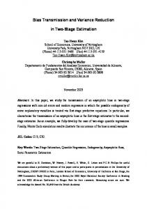
interpolating quadratic polynomial to three points, at 0.005, 0.5, 0.995; (b) we fitted an interpolating cubic polynomial to four points, at 0.005, 0.335, 0.665, 0.995; (c) instead of interpolating, we used least squares to fit a quadratic curve on 100 points at ui = (i + 0.5)/100, for i = 0, . . . , 99 (the function values were estimated from 100 simulation runs at each of these points); (d) we fitted a cubic polynomial by least squares to the same 100 points; (e) we fitted a cubic spline to these 100 points; (f) we fitted a smoothing cubic spline to 50 points. With the latter method, a constraint is imposed on the root mean square error at the selected points (this is called the smoothing factor) and the algorithm find the smoothest possible spline that satisfies the constraint. Figure 1 shows the quadratic and cubic interpolations (a) and (b), for the three functions, with black points representing results of pilot runs. Figure 2 gives the quadratic and cubic polynomial least-squares fits (c) and (d). The cubic polynomial least-squares fit (d) and the splines (e) and (f) (not shown due to lack of space) match the points a bit better and are about equally good between themselves. The plots give an idea of how β ∗ (u), σc (u), and σ (u) behave as functions of u. The optimal CV coefficient β ∗ (u), which has the same sign as Cov[C, X|U = u], is positive for small u and negative for large u. This can be explained intuitively as follows: when u is small, the load on the system is small and the agents are not very busy, so a small increase in the number of arrivals tends to increase G(s0 ). If u is large, on the other hand, the agents are occupied most of the time, so a few more arrivals increases the waiting time of several calls and tends to decrease the number of calls answered with s0 seconds. The functions σc and σ , on the other hand, increase sharply when u approaches 1, which means that the estimators have much more variance when the arrival rate is very large (the system is highly loaded). Table 3 presents the results of a simulation experiment with n = 104 replications divided into 100 strata. We compare the empirical variances with the following three methods for estimating the functions: a quadratic fit with three points, a quadratic least squares approximation with 50 points, and a cubic smoothing spline with 50 points. The smoothing splines are not really doing better for this example and they require more overhead to estimate the

σ˜ c (u)du = σ0 + σ1 /2 + σ2 /3,

so that it gives a quadratic approximation of R σc (u)/ 01 σc (u)du. The optimal allocation to any stratum is easy to obtain after this standardization: it is the average of the standardized function over the stratum, multiplied by m = n/k. In case where we use stratification without the CV, the optimal allocation to strata can be estimated in the same way, except that there is no β (u). The function σc2 (u) is replaced by σ 2 (u) = Var[X | U = u]. Note that this function σ (u) differs from σc (u), so it must be approximated separately and the optimal allocation is different. Based on pilot runs with n0 = 200 per testing point, we obtained the quadratic approximations for β , σc , σ given in Table 2. We ran a simulation experiment with n = 104 and k = 100 strata. Our estimates of the terms Var[X¯n ], Var[X¯so,n ], (1/nk) ∑ks=1 (σs − σ¯ )2 , and (1/nk) ∑ks=1 (µs − µ)2 in the variance decomposition (the first term is the sum of the three other) are given in Table 3. In comparison with standard Monte Carlo, the variance is reduced by a factor of 28.1 for proportional allocation without CV; 35.4 for with optimal allocation without CV; 35.8 for with proportional allocation with CV; 60.4 for with optimal allocation with CV. Another (simpler) option that bypasses all functional estimations is to use stratification with proportional allocation, combined with the CV with a constant coefficient β . For this case, we find that the optimal β is approximately 0.45. This is labeled “CV, β const” in the table. The variance is reduced by a factor of 30.6. We made further experiments to see if we could improve the quality of approximation of the functions β (u), σc (u), and σ (u). We tried the following alternatives: (a) we fitted an

607

L’Ecuyer and Buist

(i) β ∗ (u)

(ii) σc (u)

(iii) σ (u)

Figure 1: The Functions β ∗ (u), σc (u), and σ (u) Approximated by Polynomial Interpolation

(i) β ∗ (u)

(ii) σc (u)

(iii) σ (u)

Figure 2: The Functions β ∗ (u), σc (u), and σ (u) Approximated by Least Squares on 100 Points

function with pilot runs. Selection of the smoothing factor is also not automatic.

parameter, because we want to analyze what happens when the size of the change converges to zero.

4

4.1 Sensitivity to the Mean Service Time

COMPARING SYSTEMS WITH COMMON RANDOM NUMBERS

The service times in our model are i.i.d. gamma(α, γ), with mean α/γ and variance α/γ 2 . In the base configuration, we have α = 1 and γ = γ1 = 1/100. (With α = 1, the service times are exponential.) We want to study the effect of changing slightly the second parameter to γ = γ2 = γ1 /(1 − δ ) for a small δ . The effect of this is to multiply the mean service time by 1 − δ while keeping the coefficient of variation unchanged. The distribution of X = G(s0 ) and its expectation, µ(γ) = Eγ [X], now depend on γ. Suppose we want to estimate µ(γ2 ) − µ(γ1 ).

We now examine a situation where we want to compare two very similar configurations of the call center. This is often required in optimization settings and for sensitivity analysis. Configuration 1 (the base configuration) is the same as in the previous section. In Configuration 2, we may have a slightly different number of agents in one or more periods, or slightly different parameter values for one of the distributions (e.g., service times, patience times, arrival process). Here, we consider a small change in a parameter of the service time distribution. We have selected a continuous

608

L’Ecuyer and Buist Table 3: Stratification with a Control Variate: Variance Comparisons

X¯n nVar[X¯n ] nVar[X¯sp,n ] nVar[X¯so,n ] 1 k ¯ 2 k ∑s=1 (σs − σ ) 1 k 2 k ∑s=1 (µs − µ)

Quadratic interpolation No CV CV, β const. CV, β (u) 1419.48 1419.30 1418.59 77083 77158 76713 2743 2515 2142 2178 — 1269 565 — 873 74341 74643 74571

We simulate n days at each server speed. Let X1,i and X2,i be the realizations of G(s0 ) on day i, with γ = γ1 and γ = γ2 , respectively. Define ∆i = X2,i − X1,i and let ∆¯ n = (1/n) ∑ni=1 ∆i be the (crude) estimator of the difference µ(γ2 ) − µ(γ1 ). To compute X1,i and X2,i , we can use either (i) independent random numbers (IRNs) or (ii) common random numbers (CRNs), i.e., the same underlying uniform random numbers for the two values of γ (Bratley, Fox, and Schrage 1987, L’Ecuyer and Perron 1994). We have

Least squares, 50 points No CV CV, β (u) 1419.29 1418.88 77556 76529 2720 2166 2193 1294 527 872 74836 74363

Cubic spline No CV CV, β (u) 1418.64 1419.08 77312 76578 2754 2098 2181 1234 573 864 74558 74481

this reason, acceptance-rejection here maintains synchronization exactly as inversion. To check this, we actually tried replacing inversion with acceptance-rejection in the experiments described in what follows, and we found no significant difference. In our attempt to use the same random numbers at exactly the same places for both systems, we meet a difficulty with the synchronization: Due to the different service times, the abandonments will eventually not be the same for γ1 and γ2 . A given call may abandon in one system and not in the other. For such a call, the service time must be generated in the first case but does not have to be generated in the second case. In this context, we can generate service times:

Var[∆i ] = Var[X1,i ] + Var[X2,i ] − 2Cov[X1,i , X2,i ]. With IRNs, the covariance term is zero. The aim of CRNs is to make this covariance positive. By using the same random numbers at the same places for both systems as far as this is achievable, the responses X1,i and X2,i are expected (intuitively, at least) to be strongly positively correlated, especially if γ1 and γ2 are close. To see how the same random numbers can be used at approximately the same places in this example, we distinguish four types of random numbers: Those used to generate (1) the busyness factor in the morning; (2) the interarrival times; (3) the service times; and (4) the patience times. To make sure that the same sequences of random numbers are employed within each category, we attach a different random number stream to each category. We initialize these four generators to the same seeds for both server speeds and we generate all random variates by inversion. Do we really need to use inversion to maintain the synchronization for the CRNs? For this particular example, the answer is no. The only place where this could make a difference is the generation of service times, because for the other random variates, nothing is changed across the two configurations. For a general gamma distribution, inversion is quite time-consuming; much faster acceptance-rejection methods are available. One such method, implemented in SSJ, generates a gamma random variable of mean 1 with the required shape parameter α, then multiplies the value by the desired mean. In our example, since only the scale parameter is changed, the acceptance-rejection part of the algorithm does exactly the same thing for both configurations; only the multiplication by the desired mean changes. For

(a) (b)

for all calls (the abandoned calls will have unused service times), or only for the calls that are actually answered.

The rationale for (a) is to make sure that the same calls have the same service times in both configurations, regardless of abandonments. The argument for (b) is for the sequence of service times that are effectively employed to be the same for both systems, even though these service times may belong to different calls because of different abandonment decisions. So if a call has a very long service time for parameter γ1 , this very long service time will also appear (perhaps for another call) for γ2 under (b). Under (a), this long service time could be unused for γ2 . Likewise, the patience time can be generated: (c) (d)

for all arriving calls, to maintain synchronization, or only for the calls whose service does not start immediately upon arrival.

By combining these choices, we obtain four different possibilities for the synchronization strategy, and it is unclear a priori which one is best. Table 4 reports empirical results for δ = 0.1, 0.01, and 0.001, with n = 104 . This corresponds to a reduction of the mean service time by 10%, 1%, and 0.1%, respectively. The table gives the sample mean and the sample variance of

609

L’Ecuyer and Buist Table 4: Effect of Change in the Mean Service Time for the Call Center, with CRNs, for n = 104

Method IRN (a + c) IRN (a + d) IRN (b + c) IRN (b + d) CRN, no sync. (b + d) CRN (a + c) CRN (a + d) CRN (b + c) CRN (b + d)

δ = 0.1 c i] ¯∆n Var[∆ 76.93 192680 76.57 192374 76.96 192034 77.14 192495 76.08 11036 78.75 9307 78.78 9502 78.73 9714 78.90 9646

the ∆i ’s for simulations with independent random numbers (IRNs), simulations with CRNs without synchronization, and simulations with CRNs with the different types of synchronizations just described. For CRNs without synchronization, we just took all the random numbers needed in the simulation sequentially from a single stream instead of from four different streams, and we generated random variates only when they were needed (strategy (b + d)). Thus, for example, an inter-arrival time for one system configuration could be generated from the same random number as a service time for the other configuration. All the pairs c i ]) in the table were obtained by independent (∆¯ n , Var[∆ simulations. With any of the four combinations of synchronization approaches, CRNs reduce the variance by a huge factor. The smaller δ is, the more the variance is reduced. With IRNs, we have Var[∆i ] = Var[X1,i ] + Var[X2,i ] ≈ 2 Var[Xi ], so the variance does not depend much on δ . (It is slightly larger for δ = 0.1 because Var[X2,i ] is significantly larger in that case.) The difference between the four IRN results is just noise. With CRNs, the variance diminishes rapidly when δ → 0. A theoretical analysis of the convergence is provided in Section 4.2. When δ → 0, E[∆i ] becomes closer to 0 and thus harder to estimate. When δ is very small, the finite-difference estimators with IRNs are practically useless (too noisy), whereas those with CRNs remain viable. CRNs with (b + d) without synchronization reduces the variance much less than the good synchronization schemes, but nevertheless improves over IRNs by a significant factor. Understanding exactly why it works would require further investigation, but most of the explanation might be that (i) it takes some time before the synchronization is lost and (ii) the important variable Bi is always generated with the same random number, and thus takes a common value for both systems. With strategy (a + c), it turns out that for this particular example, synchronization is maintained across the two systems even with a single stream, because

δ = 0.01 c i] ¯∆n Var[∆ 7.48 160486 7.00 160168 7.16 159605 7.34 159970 6.71 2417 8.48 122 8.51 389 8.14 237 8.42 312

δ = 0.001 c i] ∆¯ n Var[∆ -0.135 157745 -0.560 157592 -0.216 156794 -0.215 157136 0.203 1979 0.862 5 0.786 197 0.821 21 0.819 81

the two systems get a common value of Bi and the same sequence of arrival events, each call requires exactly three random numbers upon arrival, and no random numbers are needed anywhere else. For this reason, CRNs with a single stream give the same variance reduction as CRNs with the four different streams as described earlier. Between the synchronization strategies for the CRNs, the (a + c) combination is the best performer, followed by (b + c). So it is better in this example to generate service and patience times for all calls, and simply discard the values that are not needed. The choice of strategy makes a significant difference when δ is very small, but not much when δ is larger (e.g., 0.1). We must underline that this observation should not be taken as a general rule: there are similar situations where the best synchronization strategy would be (b + d) instead. So in practice, it is worth trying and comparing. To reduce the variance further, we can combine the use of CRNs with stratification and a CV, as in Section 3. For the CV, with CRNs, we use the number A of arrivals (not the difference in number of arrivals between the two configurations, because the number of arrivals is the same for both configurations). The functions β ∗ , σc , and σ are estimated in a similar way. Table 5 presents our results for this case, for n = 104 replications with 100 strata, with (a + c) to synchronize the random numbers. We used quadratic interpolation to estimate the functions. The empirical results indicate that combining CRNs with stratification provides an additional variance reduction by a significant factor. The CV, on the other hand, does not bring additional gain. For δ = 0.1, the variance goes down approximately from 192000 to 9300 with the CRNs and to 230 when the three methods are combined. For δ = 0.001, it goes from about 157000 to 5 with the CRNs (a + c) and to 2 with the stratification.

610

L’Ecuyer and Buist Table 5: Effect of Change in the Mean Service Time for the Call Center, with CRNs, Stratification, and CV, for n = 104 and k = 100 No CV ∆¯ n , Var[∆¯ n ], Var[∆¯ sp,n ], Var[∆¯ so,n ], 1 k ¯ 2 (σ k ∑s=1 s − σ ) , 1 k 2, (µ − µ) ∑ k s=1 s

CRN CRN CRN CRN CRN CRN

77.07 9086 464 267 197 8622

δ = 0.1 CV β const 77.00 9061 415 — — 8646

CV β (u) 77.14 9075 417 230 186 8658

No CV 8.270 121 33 18 15 88

4.2 Bound on Convergence Rate When δ → 0

δ = 0.01 CV β const 8.300 119 32 — — 87

CV β (u) 8.210 115 31 18 13 84

No CV 0.816 5.0 4.2 2.0 2.2 0.8

δ = 0.001 CV β const 0.837 5.1 4.1 — — 1.0

CV β (u) 0.808 4.9 4.1 1.9 2.1 0.8

Note that the V j ’s are independent of the S j ’s and of δ . Call j switches from bad to good service when γ1 changes to γ1 /(1 − δ ) if and only if

With CRNs, X = X(δ ) is a function of δ . If X(δ ) was a continuous function of δ with a denumerable number of nondifferentiability points with probability 1, then Var[(X(δ ) − X(0))/δ ] would be bounded by a constant when δ → 0 and we would have   ∂ g(s0 ) X(δ ) − X(0) = E lim δ ∂ δ δ =0 δ →0

W j (δ ) ≤ V j < W j .

(6)

Similarly, call j switches from good to bad service if and only if W j ≤ V j < W j (δ ).

(7)

In general, the status of call j changes if and only if

where the pathwise limit inside the expectation is the infinitesimal perturbation analysis estimator of the derivative of g(s0 ) with respect to δ (L’Ecuyer 1990, Glasserman 1991, Glasserman and Yao 1992, L’Ecuyer and Perron 1994). In that case, Var[X(δ ) − X(0)] = O(δ 2 ) when δ → 0. Here the service times change continuously with δ , but X(δ ) is a piecewise constant function of δ that takes only integer values, so it is definitely not continuous. The next proposition states that under the CRN strategy (a + c), Var[X(δ ) − X(0)] = O(δ 1−ε ) for any ε > 0 when δ → 0. This is certainly not as good as O(δ 2 ), but much better than the O(1) rate that we get with IRNs. Empirically, the rate seems even better than O(δ ): the variance for CRN with (a + c) in Table 4 is divided by much more than 10 when δ is divided by 10. Proposition 1 We have Var[∆] = O(δ 1−ε ) where the hidden constant depends on ε but not on δ . The main ingredient in our proof of this proposition is a lemma that bounds the probability that X(δ ) 6= X(0), as a function of δ . For this, we need some notation. In the original model (δ = 0), the service time of the jth call (by order of arrival) is S j = G−1 (U j ) where G is the gamma(α, γ) distribution function and the U j ’s are i.i.d. U(0, 1). Let T j denote the arrival time of call j, Pj its patience time, and W j the time at which it is answered. Multiplying the parameter γ by 1/(1 − δ ) changes the service time from S j to S j (δ ) = (1 − δ )S j , and the answering time from W j to W j (δ ). Let D j = |W j − W j (δ )|. This call has good service in the original model if and only if W j ≤ V j , where V j = T j + min(Pj , s0 ) is its virtual threshold time (VTT).

min{W j ,W j (δ )} ≤ V j < max{W j ,W j (δ )}.

(8)

Let λ¯ (u) be the maximum arrival rate during the day conditional on B = b = FB−1 (u). Let Pu and Eu denote the corresponding conditional probability and conditional expectation. Lemma 1 Conditional on B = b = FB−1 (u), we have Pu [X(δ ) 6= X(0)] ≤ Eu [A2 ]α λ¯ (u)δ /γ + Eu [A3 ]O(δ 2 ) = O(δ b3 ). Proof. Recall that the patience time is exponential with parameter ν. For a small ε > 0, a given time interval [t,t + ε) can contain one (or more) of the V j ’s only if a call arrives in the time interval [t − s0 ,t − s0 + ε) and reaches its VTT before abandoning, or if a call arrives at time x for t − s0 ≤ x ≤ t + ε and abandons during the interval [t,t + ε). The probability that one of these two events occurs is bounded by λ (t − s0 ) ε e−νs0 +

Z t

λ (x) ενe−ν(t−x) dx + o(ε)

t−s0

≤ ε λ¯ (u) + o(ε) (where the function λ¯ depends on u). This gives an upper bound on the probability that [t,t + ε] contains V j

611

L’Ecuyer and Buist

j−1

D j = |W j −W j (δ )| ≤

j−1

=

∑ Pu [A = a]

a=1

 (a − 1)a α λ¯ (u)δ + O(δ 2 a3 ) 2 γ

≤ Eu [A2 ]α λ¯ (u)δ /γ + Eu [A3 ]O(δ 2 ) = O(δ b3 ). The second equality holds because A and ξ j are independent. This completes the proof of the lemma. 2 Proof of the Proposition 1. Using Holder’s inequality with 1/p = 1 − 1/q for an arbitrary q > 1 and denoting ∆ = X(δ ) − X(0), we have

def

∑ (S` − S` (δ )) = δ ∑ S` = ξ j .

`=1



∞

for a fixed j. By integrating this with respect to t over [min{W j ,W j (δ )}, max{W j ,W j (δ )}], and taking ε → 0, we find that the probability that (8) occurs cannot exceed λ¯ (u)D j . Let J ∗ be the smallest integer j > 0 for which (8) holds, i.e, the index of the first call that switches status. If there is none, put J ∗ = ∞. For j ≤ J ∗ , we have

`=1

Combining the last two bounds, we obtain that

E[∆2 | B = b] ≤ Eu [∆2 I[∆2 > 0]] ≤ (Eu [∆2q ])1/q (Eu [I p [∆2 > 0]])1/p

Pu [J ∗ = j | W j ,W j (δ )] ≤ Pu [min{W j ,W j (δ )} ≤ V j < max{W j ,W j (δ )} | W j ,W j (δ )] ≤ λ¯ (u)D j

≤ (Eu [A2q ])1/q (Pu [∆ 6= 0])(q−1)/q

≤ 1 − exp[−λ¯ (u)D j ] ≤ 1 − exp[−λ¯ (u)ξ j ]

= O((a · b)2 (δ b3 )(q−1)/q ) where (K0 (q, u))q = Eu [A2q ] = O((a · b)2q ) is a very loose bound on E[∆2q ] that does not depend on δ . By selecting q = 1/ε, this gives

j−1

= 1 − ∏ exp[−λ¯ (u)δ S` ]. `=1

Var[∆ | B = b] ≤ E[∆2 | B = b] = O((ab)2 (δ b3 )1−ε ).

Observe that the ξ j ’s are independent of the V j ’s, because the service times are independent of the arrival process. Recall also that S` has moment generating function M(t) = E[exp[tS` ]] = (1+t/γ)−α = 1−αt/γ +α(α +1)(t/γ)2 /2+ o(t 3 ) for t near 0. Putting these pieces together, and using I to denote the indicator function, we obtain the following upper bound on the probability of a change in the number of good services during the day:

On the other hand, since ∆ is an integer, we always have ∆ ≤ ∆2 and thus E[∆ | B = b] ≤ E[∆2 | B = b] = O((ab)2 (δ b3 )1−ε ). Then, Var[∆] = E[Var[∆ | B]] + Var[E[∆ | B]] = O(a2 E[B2 (δ B3 )1−ε ])

Pu [X(δ ) 6= X(0)] ∗

≤ Pu [J < ∞]

+ O(a4 E[B4 (δ 2 B6 )1−ε ]).

∞

=

∑ Eu [I[ j ≤ A]Pu [J ∗ = j | W j ,W j (δ )]]

j=1 ∞

≤ =

Since B has bounded moments of all orders, this gives Var[∆] = O(δ 1−ε ), which completes the proof. 2 The empirical results of the previous subsection indicate that Var[∆] ∈ O(δ ), at least for the (a + c) and (b + c) synchronization strategies and with the parameters values of our numerical experiment. If ∆ was bounded by a constant K0 , then we would easily have Var[∆ | B = b] = K02 Pu [∆ 6= 0] = K02 O(δ b3 ) = O(δ ). Strictly speaking, ∆ is not bounded, but when δ is small, the probability than ∆ exceeds a few units is so small that ∆ can be considered as bounded from a practical viewpoint.


 ∑ Eu I[ j ≤ A] 1 − exp[−λ¯ (u)ξ j ]

j=1 ∞

∑ Pu [ j ≤ A]Eu

  1 − exp[−λ¯ (u)ξ j ]

j=1 ∞

=

∑ Pu [ j ≤ A]

j=1 ∞

= =

j−1

!

1 − ∏ Eu [exp[−λ¯ (u)δ S` ]] `=1

  −( j−1)α ¯ P [ j ≤ A] 1 − (1 + λ δ /γ) ∑ u

j=1 ∞

∑ Pu [ j ≤ A]

  ( j − 1)α λ¯ (u)δ /γ + O(δ 2 j2 )

ACKNOWLEDGMENTS

j=1 ∞

=

a   P [A = a] u ∑ ∑ ( j − 1)α λ¯ (u)δ /γ + O(δ 2 j2 )

a=1

= K0 (q, u) · O((δ b3 )(q−1)/q )

This research has been supported by Grants OGP-0110050 and CRDPJ-251320 from NSERC-Canada, and a grant from Bell Canada via the Bell University Laboratories,

j=1

612

L’Ecuyer and Buist AUTHOR BIOGRAPHIES

to the first author. The second author benefited from an Industrial Scholarship from NSERC-Canada and the Bell University Laboratories.

PIERRE L’ECUYER is Professor in the D´epartement d’Informatique et de Recherche Op´erationnelle, at the Universit´e de Montr´eal, Canada. He holds the Canada Research Chair in Stochastic Simulation and Optimization. His main research interests are random number generation, quasi-Monte Carlo methods, efficiency improvement via variance reduction, sensitivity analysis and optimization of discrete-event stochastic systems, and discrete-event simulation in general. He is currently Associate/Area Editor for ACM TOMACS, ACM TOMS, and Statistical Computing. He obtained the prestigious E. W. R. Steacie fellowship in 1995-97 and a Killam fellowship in 2001-03. His recent research articles are available on-line from his web page: .

REFERENCES Avramidis, A. N., A. Deslauriers, and P. L’Ecuyer. 2004. Modeling daily arrivals to a telephone call center. Management Science 50 (7): 896–908. Bratley, P., B. L. Fox, and L. E. Schrage. 1987. A guide to simulation. Second ed. New York: Springer-Verlag. Buist, E., and P. L’Ecuyer. 2005. A Java library for simulating contact centers. In Proceedings of the 2005 Winter Simulation Conference, 556–565: IEEE Press. Cez¸ik, M. T., and P. L’Ecuyer. 2006. Staffing multiskill call centers via linear programming and simulation. Management Science. To appear. Cochran, W. G. 1977. Sampling techniques. Second ed. New York: John Wiley and Sons. Gans, N., G. Koole, and A. Mandelbaum. 2003. Telephone call centers: Tutorial, review, and research prospects. Manufacturing and Service Operations Management 5:79–141. Glasserman, P. 1991. Gradient estimation via perturbation analysis. Norwell, MA: Kluwer Academic. Glasserman, P., and D. D. Yao. 1992. Some guidelines and guarantees for common random numbers. Management Science 38 (6): 884–908. Glynn, P. W., and R. Szechtman. 2002. Some new perspectives on the method of control variates. In Monte Carlo and Quasi-Monte Carlo Methods 2000, ed. K.-T. Fang, F. J. Hickernell, and H. Niederreiter, 27–49. Berlin: Springer-Verlag. Lavenberg, S. S., and P. D. Welch. 1981. A perspective on the use of control variables to increase the efficiency of Monte Carlo simulations. Management Science 27:322– 335. L’Ecuyer, P. 1990. A unified view of the IPA, SF, and LR gradient estimation techniques. Management Science 36 (11): 1364–1383. L’Ecuyer, P. 2006. Stochastic simulation. Notes for a graduate simulation course. L’Ecuyer, P., and E. Buist. 2005. Simulation in Java with SSJ. In Proceedings of the 2005 Winter Simulation Conference, 611–620: IEEE Press. L’Ecuyer, P., and G. Perron. 1994. On the convergence rates of IPA and FDC derivative estimators. Operations Research 42 (4): 643–656. Whitt, W. 1999. Dynamic staffing in a telephone call center aiming to immediately answer all calls. Operations Research Letters 24:205–212.

ERIC BUIST is a PhD Student at the Universit´e de Montr´eal. His main interests are software engineering, object-oriented programming, and simulation. He is currently working on the development of flexible and efficient tools for the simulation of contact centers. His e-mail address is .

613