However non- deterministic knowledge like preference and frequency seems difficult to represent as logic. Bayesian inference can reflect such knowledge on a.
Variational Bayes inference for logic-based probabilistic models on BDDs Masakazu Ishihata, Yoshitaka Kameya, and Taisuke Sato Tokyo institute of Technology 2-12-1 Ookayama, Meguro-ku Tokyo, Japan {ishihata,kameya,sato}@mi.cs.titech.ac.jp
Abstract. Statistical abduction is an attempt to define a probability distribution over explanations derived by abduction and to evaluate them using their probabilities. In statistical abduction, deterministic knowledge like rules and facts are described as logic formulas. However nondeterministic knowledge like preference and frequency seems difficult to represent as logic. Bayesian inference can reflect such knowledge on a prior and variational Bayes (VB) is known as an approximation method for it. In this paper, we propose VB for logic-based probabilistic models and show that our proposed method is efficient in evaluating abductive explanations about failure in a logic circuit and a metabolic pathway.
1
Introduction
Abduction is one of logical inference to find explanations E from knowledgebase KB for an observation O such that KB ∧ E ` O and KB ∧ E is consistent. Statistical abduction defines a probability distribution over explanations and attempts to evaluate them by their probabilities. A couple of frameworks for statistical abduction have been proposed [1, 2] but they have restrictions on KB to realize efficient probability computation and learning. To relax these restrictions, the BO-EM algorithm which is an EM algorithm for propositional logic-based probabilistic models (PBPMs) was proposed [3]. A PBPM p(b|θ) is a joint distribution over boolean random variables b and defines probabilities for any boolean formulas. Probabilistic events (observations O) in a PBPM p(b|θ) are described as boolean formulas (explanations E) and a parameter θ can be learned by BO-EM in a dynamic programming manner on a BDD representing E. In statistical abduction, deterministic knowledge like rules and facts is described by logic as KB. However, non-deterministic knowledge like preference and frequency is difficult to represent by logic. To explicitly reflect such knowledge, Bayesian inference which is a method for statistical inference is useful. It assumes θ as a random variable and introduces a prior p(θ|α) corresponding to preference or frequency of θ. Then, it computes a posterior p(θ|O, α) which is a modified distribution by observations O. However the computation of the posterior requires complex summation and integration. Variational Bayes (VB) inference is an deterministic approximation of Bayesian inference and the VBEM algorithm [4] is known as an EM like iterative computation for VB.
In this paper, we propose a VB-EM algorithm for PBPMs which is a generalization of the BO-EM algorithm for VB. We show that the complexity of our method is the same as BO-EM and also show that it runs efficiently in evaluating abductive explanations for a logic circuit and a metabolic pathway.
2
Preliminaries
2.1
Propositional logic based probabilistic models (PBPMs) ∑Mj Mj Let θj ≡ {θjv }v=1 (0 ≤ θjv ≤ 1, v=1 θjv = 1) be a parameter of a categorical i distribution Cat (θj ) corresponding to an Mj -sided dice. Also let xi ≡ {xiv }N v=1 ∑Ni (xiv ∈ {0, 1}, v=1 xiv = 1) be a 1-of-Ni expression of a value drawn from Cat (θji ) (1 ≤ ji ≤ M ). We use vi to denote v such that xiv = 1. Then, the ∏Ni xiv probability of xi is computed by p(xi | θji ) = v=1 θji v = θji vi . Let x and θ be M {xi }N and {θ } , respectively. Then, the probability of x is computed by j j=1 i=1 p(x | θ) =
Mj M ∏ ∏
σ
θjvjv
(x)
∑
σjv (x) ≡
,
j=1 v=1
xiv .
i:ji =j
Let f be a function of x. Then, a boolean function fy (x) ≡ “f (x) = y” corresponds to a probabilistic event and its probability is computed as p(fy | θ) = ∑ 0 0 x fy (x)p(x | θ). We use “xi = v” to denote xiv = 1 and xiv = 0 (v 6= v). Then, fy can be represented as a boolean formula as follows: ∨ ∧ fy = “xi = vi ”. x:f (x)=y xi ∈x
Probabilistic events “xi = v” and “xi = v 0 ” (v 6= v 0 ) depend on each other. However, they can be described as a boolean formula of independent boolean random variables b ≡ {biv | biv ≡ “xi ≤ v | xi ≥ v”, 1 ≤ i ≤ N, 1 ≤ v < Ni } as follows [3]: { ∧v−1 biv ∧ v0 =1 ¬biv0 1 ≤ v < Ni , “xi = v” ≡ ∧v−1 0 v = Ni v 0 =1 ¬biv where the probability of biv is defined as follows: θj v p(biv |θ) ≡ i , φji v
φj ,v+1 p(¬biv |θ) ≡ i , φji v
φjv ≡
Then, the probability of “xi = v” (1 ≤ v < Ni ) is computed by p(“xi = v” | θ) = p(biv | θ)
j−1 ∏
p(¬biv0 | θ)
v 0 =1
=
v−1 θji v ∏ φji ,v0 +1 φ ji v 0 φji v0 v =1
= θji v (= p(xi = v | θ)) .
Mj ∑ v 0 =v
θjv .
Consequently, p(x | θ) can be computed by p(b | θ). The propositionalized distribution p(b | θ) is called a propositional logic-based probabilistic model (PBPM) for p(x | θ) and defines probabilities for any boolean formulas in b. 2.2
Maximum likelihood estimation and the EM algorithm
We assume that a probabilistic event fy is sampled from p(fy , x | θ) and that x and θ are unobservable. Maximum likelihood estimation (MLE) estimates the parameter θ as θˆ ≡ argmaxθ p(fy | θ). When there are hidden variables like x, it is popular to use the EM algorithm for MLE. It iterates the following update: (t+1)
θjv
E[σjv (x)]p(x|fy ,θ(t) ) = ∑Mj , v 0 =1 E[σjv 0 (x)]p(x|fy ,θ (t) )
(1)
but it only converges to a local maximum of p(fy | θ). The above expectations E[σiv (x)]p(x|fy ,θ(t) ) can be computed using the PBPM p(fy , b | θ). The BO-EM algorithm which is an EM algorithm for PBPMs computes them on a BDD representing fy in time linear in the BDD size [3]. 2.3
Variational Bayes inference and the VB-EM algorithm
Whereas MLE considers a parameter θ as an unknown constant and estimates it as what maximizes p(fy | θ), Bayesian inference considers θ as a random variable and computes a distribution of θ given fy . A prior distribution p(θ | α) is given beforehand and a posterior distribution p(θ | fy , α) is computed by ∑∫ p(θ | fy , α) = p(fy | θ)p(θ | α)/p(fy | α), p(fy | α) = p(fy , x | θ)p(θ | α)dθ. x
While the number of possible x is too huge, it is difficult to compute the above posterior. The variational Bayes (VB) inference is known as a deterministic approximation of Bayesian inference. It approximates a joint posterior p(x, θ | fy , α) by a variational distribution q(x, θ) = q(x)q(θ). Using q(x) and q(θ), the log marginal likelihood ln p(fy | α) can be obtained as a sum of a variational free energy (VFE) F[q] and the Kullback-Leibler (KL) divergence KL(q||p) as follows: ∑∫ ln p(fy | α) = q(x)q(θ) ln p(fy | α)dθ x
=
∑∫
q(x)q(θ) ln
x
p(x, fy , θ | α)q(x)q(θ) dθ p(x, θ | fy , α)q(x)q(θ)
= F[q] + KL(q||p) , where ∑∫ ∑∫ q(x)q(θ) p(x, fy , θ|α) q(x)q(θ) ln q(x)q(θ) ln dθ, KL(q||p) = dθ. F[q] = q(x)q(θ) p(x, θ|fy , α) x x
Since KL(q||p) is non-negative, F[q] gives a lower bound of ln p(fy | α). Maximizing F[q] with respect to q results in minimizing KL(q||p). The variational Bayes EM (VB-EM) algorithm is an EM like iterative algorithm for VB inference [4]. It attempts to maximize F[q] by iterating the following updates: ) ( q (t+1) (x) ∝ exp E[ln p(x, fy | θ)]q(t) (θ) , (2) ( ) q (t+1) (θ) ∝ p(θ | α)exp E[ln p(x, fy | θ)]q(t+1) (x) . (3) The above updates are repeated until F[q] converges. When converged, the VBEM algorithm outputs q(θ) as an approximation of the posterior p(θ | fy , α).
3
Proposed method
3.1
Bayesian inference for PBPMs
k Let αk ≡ {αkv }L v=1 (αkv > 0) be a parameter ( ) of a Dirichlet distribution Dir (αk ). We assume θj is sampled from Dir αkj . Then, the prior distribution p(θ | α) (α ≡ {αk }L k=1 ) is represented as a product of Dirichlet distributions:
p(θ|α) =
M ∏
p(θj |αkj ),
j=1
∏Lk Mj 1 ∏ αkv −1 v=1 Γ(αkv )) . p(θj |αk ) = θjv , Z (αk ) ≡ (∑ Lk Z (αk ) v=1 α Γ v=1
kv
Because a Dirichlet distribution is a conjugate prior of a categorical distribution, the posterior p(θ | fy , α) becomes a sum of products of Dirichlet distributions: p(θ | fy , α) ∝
∑ x
3.2
M ∏
Mj ∏ αk v +σjv (x)−1 1 ( ) fy (x) θjv j . Z αkj v=1 j=1
VB-EM algorithm for PBPMs
We propose a VB-EM algorithm for PBPMs. By substituting the definitions of p(x | θ) and p(θ | α) into (2) and (3), we get the following updates: q
(t+1)
(x) ∝
Ni ( N ∏ ∏
(t+1) θ˜iv
)σiv (x) ,
q
(t+1)
(θ) ∝
i=1 v=1
M ∏ j=1
( Z
1 (t+1) α ˜j
(t+1) (t+1) where θ˜iv and α ˜ kv are defined as follows: ( (M )) ( ) ∑i (t) (t+1) (t) (t+1) θ˜ ≡ exp Ψ α ˜ −Ψ α ˜ 0 , α ˜ ≡ αk iv
kj v
kj v
jv
jv
)
Mj ∏
(t+1)
α ˜
θjvjv
−1
,
v=1
+ E[σjv (x)]q(t+1) (x) ,
v 0 =1 d ln Γ(x). The point here where Ψ(x) is the digamma function defined by Ψ(x) ≡ dx is that the above expectation E[σij (x)]q(k+1) (x) can be computed by substituting
(t+1) (t) θ˜iv into θiv in the computation of E[σjv (x)]p(x|fy ,θ(t) ) in (1). As mentioned in Section 2, the BO-EM algorithm [3] computes E[σjv (x)]p(x|fy ,θ(t) ) by using p(fy , b | θ) which is a PBPM for p(fy , x | θ) and a BDD which represents fy in linear time to the BDD size. Consequently, the VB-EM algorithm for PBPMs can also be executed on the BDD in the same time and space complexity as the BO-EM algorithm. Due to space limitations, the detail of our proposed algorithm is omitted.
4 4.1
Experiments Artificial problem: diagnosis for failure in a logic circuit
We apply our method to a diagnosis for a 3-bit adder circuit involving error gates [1, 3]. An error gate is stochastically stuck at 0 or 1. The task is to find error gates in the circuit from observations that pairs of input and output values. The previous approach [3] learns probabilities of gates being stuck by the BO-EM algorithm and predicts where error gates are by using their probabilities. In this experiment, we assume the average rate of a gate being normal, stuck at 0 and stuck at 1 is given as non-deterministic knowledge. To reflect the knowledge in prediction, we use our proposed method and obtain gate probabilities. We compare the prediction accuracy of our approach with that of the previous approach. The left side of Fig. 1 respectively shows precision, recall and F-measure of the previous approach and the right shows ours. These quantities are computed by predicting error gates in 10,000 randomly-generated 3-bit adder circuits while changing the number of observations N = 10, 50, 100. The result shows that our approach achieves higher F-measure value than the previous one and also shows that introducing non-deterministic knowledge is efficient in prediction. 4.2
Real problem: hypotheses finding in a metabolic pathway
Inoue et al. applied statistical abduction to find and rank explanations for a metabolic pathway data [3]. According to them there are two important reactions which tend to be inhibited and the knowledge is used to evaluate their ranking result. To explicitly reflect such knowledge in ranking, we apply our proposed method to ranking 66 explanations derived by them. Fig. 2 shows that explanations which have top 20 high probabilities. 22 out of 66 explanations are considered good because they include the above mentioned two important reactions as inhibited. The result shows that 16 out of top 20 explanations are good and also that our method can explicitly reflect non-deterministic knowledge in ranking explanations.
5
Conclusions and Related work
We propose a variational Bayes inference for PBPMs. In the context of Bayesian inference for statistical abduction, deterministic knowledge is described
1 0.95
BO-EM
Precision Recall F-measure
Proposed method
1.2e-02 Good explanations 1.0e-02
0.9 0.85 Probability
8.0e-03
0.8 0.75 0.7
6.0e-03
4.0e-03
0.65 2.0e-03
0.6 0.55
10
50
100
10
50
# observations
Fig. 1. Predicting result
100
0.0e+00
44 30 26 33 59 14 2 65 49 21 34 48 63 20 51 23 62 5 60 3 Explanation ID
Fig. 2. Ranking result
as logic formulas whereas non-deterministic knowledge is represented as a prior distribution. We apply our proposed method to a diagnosis for failure in a logic circuit and to evaluating explanations for a metabolic pathway data. The experimental results show that introducing non-deterministic knowledge as a prior makes both of prediction and ranking results better. PRISM [2] is a probabilistic extension of Prolog and variational Bayes inference for it has already proposed [5]. However, PRISM has the exclusiveness condition for explanations to realize efficient probability computation. Our proposed method can eliminate the exclusiveness condition because it can deal with any boolean formulas. ProbLog [6] which is another probabilistic extension of Prolog also employs a BDD-based parameter learning algorithm [7]. However, variational Bayesian inference for ProbLog has not yet been proposed to our knowledge.
References 1. Poole, D.: Probabilistic Horn abduction and Bayesian networks. Artificial Intelligence 64(1) (1993) 81–129 2. Sato, T., Kameya, Y.: Parameter Learning of Logic Programs for Symbolicstatistical Modeling. Journal of Artificial Intelligence Research 15 (2001) 391–454 3. Ishihata, M., Kameya, Y., Sato, T., Minato, S.: An EM algorithm on BDDs with order encoding for logic-based probabilistic models. In: Proc. of ACML’10. (2010) 4. Beal, M., Ghahramani, Z.: The Variational Bayesian EM Algorithm for Incomplete Data: with Application to Scoring Graphical Model Structures. Bayesian Statistics 7 (2003) 5. Sato, T., Kameya, Y., Kurihara, K.: Variational Bayes via propositionalized probability computation in PRISM. Annals of Mathematics and Artificial Inteligence 54(1-3) (2009) 135–158 6. De Raedt, L., Kimming, A., Toivonen, H.: ProbLog: A probabilistic Prolog and its application in link discovery. In: Proc. of IJCAI’07. (2007) 2468–2473 7. Gutmann, B., Thon, I., De Raedt, L.: Learning the parameters of probabilistic logic programs from interpretations, Department of Computer Science, K.U.Leuven (2010)