Patrick Pérez. Microsoft Research. Cambridge, CB3 0FB, UK ...... [13] S. Waterhouse, D. MacKay, and T. Robinson. Bayesian methods for mixtures of experts.
Variational Inference for Visual Tracking Jaco Vermaak Cambridge University Engineering Department Cambridge, CB2 1PZ, UK
Neil D. Lawrence University of Sheffield 211 Portobello Street Sheffield, S1 4DP, UK
Abstract The likelihood models used in probabilistic visual tracking applications are often complex non-linear and/or nonGaussian functions, leading to analytically intractable inference. Solutions then require numerical approximation techniques, of which the particle filter is a popular choice. Particle filters, however, degrade in performance as the dimensionality of the state space increases and the support of the likelihood decreases. As an alternative to particle filters this paper introduces a variational approximation to the tracking recursion. The variational inference is intractable in itself, and is combined with an efficient importance sampling procedure to obtain the required estimates. The algorithm is shown to compare favourably with particle filtering techniques on a synthetic example and two real tracking problems. The first involves the tracking of a designated object in a video sequence based on its colour properties, whereas the second involves contour extraction in a single image.
1. Introduction Visual tracking involves the detection and recursive localisation of objects in video sequences. Depending on the application a wide variety of objects may be of interest, including people [6], cars [7], etc. Recursive tracking principles may also be applied to the tracking of fictitious objects in single images, leading to e.g. contour extraction algorithms [9]. Localisation of objects based on image data is a difficult problem. This is mainly due to the many degrees of freedom that characterise these problems, including variations due to changes in object pose and illumination, full and partial object occlusions, and many more. These factors all increase the uncertainty about the exact object location and configuration. To accurately capture this uncertainty a probabilistic framework is required. Within a tracking context one particularly popular approach is Bayesian Sequential Estimation. This framework
1063-6919/03 $17.00 © 2003 IEEE
Patrick P´erez Microsoft Research Cambridge, CB3 0FB, UK
allows the recursive estimation of a time-evolving distribution that describes the object state conditional on all the observations seen so far, commonly known as the filtering distribution. It requires the definition of a Markovian dynamical model that describes how the state evolves, and a model to evaluate the likelihood of a hypothesised state giving rise to the observed data. This, in theory, is sufficient to allow recursive estimation of the filtering distribution. However, as will be evident, the likelihood models for tracking often lead to intractable inference, requiring approximation techniques. One particularly popular approximation method is Sequential Monte Carlo Estimation, otherwise known as Particle Filters [4]. Its popularity stems from its simplicity, generality and success over a wide range of challenging problems. It represents the filtering distribution with a set of samples, or particles, and associated importance weights, which are then propagated through time to give approximations of the filtering distribution at subsequent time steps. It requires only the definition of a suitable proposal distribution from which new particles can be simulated, and the ability to evaluate the likelihood and dynamical models. Particle methods, however, suffer from the curse of dimensionality. This is further aggravated by the sharply peaked likelihoods common to many visual tracking problems. Due to the finite sample approximation only a small number of particles, if any, are generated in regions of high likelihood. In the best case this leads to a loss of generality, i.e. the filtering distribution is represented by only a small number of distinct particles (often only one), and in the worst case, a complete loss of track. This shortcoming has been acknowledged before, and many strategies have been proposed to circumvent the problem. A naive, but common, approach is to artificially broaden the likelihood function. The resulting increase in the likelihood support makes detection more probable, but discards important information about the object location and configuration. A more elegant technique based on this idea is the Annealed Particle Filter [3]. At each time step particles are guided to areas of high likelihood
by an annealing schedule that starts from a broad version of the likelihood, which is progressively refined until the target likelihood is achieved. Other strategies can be categorised as those attempting to build better proposal distributions (e.g. the Unscented Particle Filter [12]), those that reduce the size of the space explored by particles (e.g. RaoBlackwellisation [1]), or those that perform a local exploration of the likelihood surface before predicting new particles (e.g. the Auxiliary Particle Filter [11] and Local Monte Carlo methods [8]). However, not all these strategies are generally applicable to visual tracking problems. PSfrag replacements As an alternative to the sample based approximation provided by particle filters this paper proposes a variational approximation to the filtering distribution. Based on this, an EM-like algorithm is derived to estimate the filtering distribution recursively through time. The approach is derived for arbitrary likelihood models, and requires only that the likelihood can be evaluated up to a constant factor. The variational inference is intractable, and is combined with an efficient importance sampling procedure to obtain the desired estimates. The variational algorithm effectively circumvents the problems associated with particle filters by adapting the importance distribution throughout the update procedure. The remainder of the paper is organised as follows. Section 2 introduces the model used for tracking. Section 3 describes the general Bayesian sequential estimation procedure. Section 4 introduces particle filters as an approximation technique for Bayesian sequential estimation. As an alternative to particle filters, Section 5 develops a variational approximation to the sequential estimation problem. Section 6 compares the performance of the variational algorithm with that of the standard and annealed particle filters on a synthetic example and two real tracking problems. The first involves the tracking of a designated object in a video sequence based on its colour properties, whereas the second involves contour extraction in a single image. Finally, Section 7 summarises the main findings of the paper.
2. Model Description The proposed model is graphically depicted in Figure 1. The state at time t is denoted by xt , and is assumed to be comprised of all the variables of interest pertaining to the object being tracked, e.g. location, scale, orientation, etc. The uncertainty about the state is captured by assuming it to be Gaussian distributed, i.e. p(xt |µt , λt ) = N(xt |µt , λt ), where µt and λt respectively denote the mean vector and precision matrix. To further capture the uncertainty about the state distribution the mean vector and precision matrix
are assumed to be unknown random variables to be estimated alongside the state. This endows the model with the flexibility to capture the uncertainty about the state variables, together with any correlations that may exist among these variables.
µt−1
∗ µt ∼ N(µ∗ t , λt )
µt ∼ N(µt−1 , λ) λt ∼ Wn (S)
λt ∼ Wn∗ (S∗ t) t
variational ≈ approximation
xt ∼ N(µt , λt )
xt ∼ q N
yt
Figure 1. Model. Generative system model for tracking (left) and variational posterior approximation (right). In visual tracking applications it is often the case that very little is known beforehand about the object motion. It is therefore advisable to use motion models capable of capturing a wide range of motions. Even in cases where accurate motion models can be constructed a general model often performs better since large inaccuracies can result if the actual object motion deviates from that predicted by the model. Here the object motion is modelled by assuming the state mean to follow a Gaussian random walk, i.e. p(µt |µt−1 ) = N(µt |µt−1 , λ), where λ is a fixed precision matrix, set to reflect the region of uncertainty for the new estimate around the old one. Note that no generality is lost compared to the conventional approach that places the dynamics directly on the state itself. Finally, the uncertainty about the state precision matrix is captured by assuming it to be Wishart distributed, i.e. p(λt ) = Wn (λt |S), with n and S respectively the degrees of freedom and precision matrix, both assumed to be fixed. The hierarchical structure of the model effectively results in heavy-tailed dynamics on the state xt . The lower the degrees of freedom n, the heavier the tails, allowing discrete jumps in the object trajectory. For the moment the likelihood p(yt |xt ), where yt is a vector of observations, is left undefined. The tracking algorithms presented in the subsequent sections are applicable to arbitrary likelihood models, which may be nonlinear and/or non-Gaussian, and requires only that the likelihood can be evaluated up to a constant factor. The like-
lihood models for the specific tracking applications considered here are derived in Section 6 where the applications are introduced.
3. Bayesian Sequential Estimation Given the model in Section 2 the distribution of interest for tracking is the posterior p(αt |y1:t ), also known as the filtering distribution, where αt = (xt , µt , λt ) denotes the extended state, and y1:t = (y1 · · · yt ) denotes all the observations up to the current time step. This distribution can be obtained according to the recursion Z p(αt |y1:t ) ∝ p(yt |αt ) p(αt |αt−1 )p(dαt−1 |y1:t−1 ), which is initialised by some distribution for the initial state p(α0 ). Once the sequence of filtering distributions is known point estimates of the state can be obtained according to any appropriate loss function, leading to e.g. maximum a posteriori (MAP) and minimum mean square error (MMSE) estimates. The tracking recursion yields closed-form expressions in only a small number of cases. The most well-known of these is the Kalman filter for linear Gaussian likelihood and dynamical models. For models that are non-linear and/or non-Gaussian the tracking recursion is analytically intractable, and approximation techniques are required. The following two sections introduce approximation techniques applicable to the model in Section 2.
4. Particle Filters Sequential Monte Carlo methods [4], otherwise known as Particle Filters, have gained a lot of popularity in recent years as a numerical approximation to the tracking recursion for complex models. This is due to their simplicity and modelling success over a wide range of challenging applications. The basic idea behind particle filters is very simple. (i) (i) Starting with a weighted set of samples {αt−1 , wt−1 }N i=1 approximately distributed according to p(αt−1 |y1:t−1 ), new samples are generated from a suitably chosen proposal distribution, which may depend on the old state and the new (i) (i) measurements, i.e. αt ∼ q(αt |αt−1 , yt ). To maintain a consistent sample the new particle weights are set to (i)
(i)
wt ∝
(i)
(i)
(i)
(i)
(i)
(i)
5. Variational Sequential Estimation This section derives a variational approximation to the tracking recursion for the model in Section 2. Section 5.1 first gives a brief overview of variational inference, before Section 5.2 applies it to the sequential estimation algorithm.
5.1. Variational Inference
(i)
wt−1 p(yt |αt )p(αt |αt−1 ) q(αt |αt−1 , yt )
integration. From time to time it is necessary to resample the particles to avoid degeneracy of the weights (see [4] for more details). The performance of the particle filter hinges on the quality of the proposal distribution. The Bootstrap Filter [5], which is the first modern variant of the particle filter, uses the dynamical model as proposal distribution, so that the new weights become proportional to the corresponding particle likelihoods. This leads to a very simple algorithm, requiring only the ability to simulate from the dynamical model and to evaluate the likelihood. However, it performs poorly for narrow likelihood functions, especially in higher dimensional spaces. To circumvent these problems it is necessary to take more care in the design of the proposal distribution. In [4] it is proved that the optimal choice for the proposal (in terms of minimising the variance of the weights) is the posterior p(αt |αt−1 , yt ) ∝ p(yt |αt )p(αt |αt−1 ). However, this distribution and its associated weight are rarely available in closed-form. Many suboptimal strategies have been proposed to increase the efficiency of the particle filter under these circumstances, e.g. Rao-Blackwellisation [1], the Unscented Particle Filter [12], the Auxiliary Particle Filter [11], Local Monte Carlo methods [8], etc. However, not all these methods are generally applicable. One attractive suboptimal strategy is the Annealed Particle Filter, introduced in the context of visual tracking in [3]. At each time step particles are guided to areas of high likelihood by an annealing schedule that starts from a broad version of the likelihood, which is progressively refined until the target likelihood is achieved. As an alternative to particle filters the next section introduces an approximation to the filtering recursion based on variational inference. This strategy is compared with the standard and annealed particle filters on a number of visual tracking problems in Section 6.
.
The new particle set {αt , wt }N i=1 is then approximately distributed according to p(αt |y1:t ). Approximations to the desired point estimates can then be obtained by Monte Carlo
In a Bayesian setting the objective of variational inference is to find a tractable and accurate posterior approximation to an intractable posterior distribution. In this section y denotes the observed data, and α, the latent data, including any model parameters of interest. The objective is often restated as the maximisation of a lower bound on the marginal
As will be evident shortly q(µt−1 ) is Gaussian, defined as q(µt−1 ) = N(µt−1 |µ∗t−1 , λ∗t−1 ). Since the evolution for the state mean is Gaussian as well, qp (µt ) is also Gaussian, and of the form
log-likelihood, obtained as Z Z p(y, α) log p(y) = log p(y, dα) = log q(dα) q(α) Z Z ≥ q(dα) log p(y, α) − q(dα) log q(α)
qp (µt ) = N(µt |µpt , λpt ),
= LB(log p(y)),
with
where the middle line follows from Jensen’s inequality, and q(α) denotes the approximation to the posterior distribution. It is straightforward to show that Z p(α|y) log p(y) − LB(log p(y)) = − q(dα) log q(α) = KL(q(α)||p(α|y)), meaning that maximising the lower bound is equivalent to minimising the Kullback-Leibler (KL) divergence between the approximate and true posterior distributions. Here it is assumed that the approximate posterior distribution facQ torises over disjoint subsets of α, i.e. q(α) = i q(αi ). In this case it can be shown (see [13]) that the approximate posterior distributions that maximise the lower bound are of the form q(αi ) ∝ exphlog p(y, α)iQj6=i q(αj ) ,
(1)
where h·ip denotes the expectation operator relative to the distribution p. This result will be used extensively in the next section.
5.2. Variational Tracking For the model in Section 2 the tracking recursion reduces
µpt = µ∗t−1 ,
λpt = (λ∗−1 t−1 + λ
−1 −1
)
.
(4)
This is exactly equivalent to the prediction distribution of the Kalman filter before the new data is seen. With this definition for the prediction distribution all the distributions on the right hand side of (3) are now known, and variational inference for the components of the new posterior distribution can proceed according to (1). For the state mean and precision the inference leads to closed-form expressions of the form q(µt ) = N(µt |µ∗t , λ∗t ),
q(λt ) = Wn∗t (λt |S∗t ),
with µ∗t = λ∗−1 (hλt ihxt i + λpt µpt ) t λ∗t = hλt i + λpt n∗t = n + 1 −1 S∗t = (hxt xTt i − hxt ihµt iT − hµt ihxt iT + hµt µTt i + S )−1 . (5) In the above the expectations relative to the distributions q(µt ) and q(λt ) are given by + µ∗t µ∗T hµt µTt i = λ∗−1 t . t (6) Due to the general form of the likelihood the expression for q(xt ) does not yield a tractable form. However, it can be simplified to hµt i = µ∗t ,
hλt i = n∗t S∗t ,
to q(xt ) ∝ p(yt |xt )N(xt |hµt i, hλt i). p(xt , µt , λt |y1:t ) ∝ p(yt |xt )p(xt |µt , λt )p(λt ) Z × p(µt |µt−1 )p(dxt−1 , dµt−1 , dλt−1 |y1:t−1 ).
(2)
This immediately suggests an importance sampling procedure to obtain a Monte Carlo approximation to q(xt ), i.e.
As depicted in Figure 1 it is assumed that the filtering distribution can be approximated by a factorised form, i.e. p(xt , µt , λt |y1:t ) = q(xt , µt , λt ) = q(xt )q(µt )q(λt ). Using this approximation it is shown in what follows how a variational update procedure can be obtained for the tracking recursion. Substituting the variational approximation at time t − 1 into (2) and simplifying, yields p(xt , µt , λt |y1:t ) ∝ p(yt |xt )p(xt |µt , λt )p(λt )qp (µt ), (3) with Z qp (µt ) = p(µt |µt−1 )q(dµt−1 ).
q N (xt ) =
N X
(i)
wt δx(i) (dxt ),
i=1
t
with (i)
p(yt |xt ) (i) , w t = PN (j) j=1 p(yt |xt ) (7) where δx (d·) denotes the Dirac delta measure on x. Using this Monte Carlo approximation the required expectations relative to q(xt ) can be approximated as (i)
xt ∼ N(xt |hµt i, hλt i),
hxt i ≈
N X i=1
(i) (i)
w t xt ,
hxt xTt i ≈
N X i=1
(i) (i) (i)T
w t xt xt
. (8)
µ∗t = µpt , λ∗t = 2λpt ,
n∗t = n + 1, −1 + S )−1 . S∗t = (2λp−1 t
(9)
Note that once n∗t is set it does not require any further updating. The complete variational sequential estimation algorithm is summarised below. Algorithm 1 Variational Sequential Estimation • Input the prior parameters: λ, n, S. • Initialisation: set µ∗0 and λ∗0 to sensible values. • For t = 1, 2, · · · , do: − Compute the prediction distribution parameters in (4). − Initialise the variational parameters as in (9). − Compute the initial expectations in (6). − Iterate until convergence:
6. Experimental Results This section compares the performance of the variational tracking algorithm with that of the standard and annealed particle filters on a synthetic example and two real tracking problems. The first involves the tracking of a designated object in a video sequence based on its colour properties, whereas the second involves contour extraction in a single image.
6.1. Synthetic Example The purpose of the synthetic example is to establish a baseline performance comparison on a relatively difficult problem where the ground truth is known. The synthetic example considered here is representative of the problems that are difficult to solve using particle filtering techniques. The state consists of the 1D position and radius of an object of interest1 , i.e. x = (p, r). Measurements are taken on a fixed 1D grid of G points, i.e. y = (y1 · · · yG ). Measurements from gridpoints covered by the object are uniformly distributed, whereas those in the background follow a gamma distribution. More formally, ( UY (yg ) if g ∈ [p − r, p + r] p(yg |x) = (10) Ga(yg |a, b) otherwise, where Y is the region of support for the measurements. The total likelihood is obtained by assuming QGthe gridpoints to be independent, leading to p(y|x) = g=1 p(yg |x). This likelihood is non-linear in x and sharply peaked in the state space. It is representative of those encountered in visual tracking applications, e.g. [6].
· Simulate N state samples as in (7). · Compute the state expectations in (8). · Update the variational parameters according to (5). · Update the expectations in (6).
Convergence of the algorithm can be checked by monitoring the change in the variational posterior parameters, PSfrag replacements or using any other convenient convergence criterion. Each variational update step requires only very simple calculations, and the computational complexity would largely depend on the cost of evaluating the likelihood. The rate of convergence in turn depends on the efficiency of the importance sampling procedure. Since the importance distribution is adapted with the update iterations, one would expect successive sample sets to progressively cluster around areas of high posterior probability, and the effective sample size to increase.
100 90 80
Measurements
Depending on the application it may be possible to incorporate elements of the likelihood in the proposal distribution, leading to a more efficient importance sampling procedure. Only the general case is considered here. From the expressions above it is clear that the variational posterior parameters depend on expectations relative to the components of the variational posterior, which in turn depend on the variational posterior parameters, and so on. Hence these quantities can be estimated in an iterative fashion, conditional on each other, in a similar manner to the EM algorithm. The variational posterior parameters are initialised according to
70 60 50 40 30 20 10 10
20
30
40
50
60
70
80
90
Time
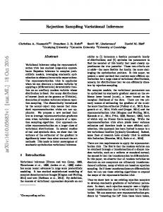
Figure 2. Synthetic data. At each time step measurements are obtained over a 1D receptor field with 100 detectors. The brightness of a pixel is proportional to the value of the measurement. The true object position and radius is also shown. 1 For
brevity the time subscript is suppressed in what follows.
100
Figure 2 shows some synthetic data for 100 time steps with Y = [0, 255] and (a, b) = (1, 0.05). The true state is superimposed on the data. This data was used to compare the performance of the tracking algorithms in terms of the average RMS state estimation error, defined as E=
M T ��1/2 1 X � 1 X� (m) (m) (pt − pbt )2 + (rt − rbt )2 , M m=1 T t=1 (m)
(m)
where (b pt , rbt ) is the state estimate at time t for the m-th replication of the experiment, with M = 10 in all cases. The fixed parameters of the model were set to λ = diag(5−2 , 1), n = 2, S = diag(10, 10), µ∗0 = [50, 10]T , λ∗0 = diag(25−2 , 10−2 ). For the standard particle filter particles were simulated from the model equations, so that the weights become proportional to the corresponding likelihood values. For the annealed particle filter the likelihood was annealed using powers ranging linearly from γ1 = 0.01 to γR = 1 over R = 20 steps at each time step. The proposal at each annealing step was formed by raising the state equations to the same power. For all three algorithms state estimates were obtained by computing the weighted average of the particles representing the state distribution. The results are presented in Figure 3. The annealed particle filter outperforms the standard particle filter, achieving the same estimation accuracy with only 5% of the particles required by the standard particle filter. This effect will be even more pronounced in higher dimensions. However, the variational algorithm emerges as the superior strategy, yielding the lowest error rate of the three algorithms for the same computational effort. PF APF VAR
PF APF VAR 1
1
10
Error
10
replacements 0
0
10
10 1
10
2
10
Sample Size
3
10
4
10
6
10
Flops per Time Step
Figure 3. Error curves. RMS state estimation error and error bars as a function of the number of particles (left) and of the average number of floating point operations per time step (right).
6.2. Object Tracking This section considers the tracking of a bounding box enclosing an object or a region of interest in a video se-
quence. However, more general object models can easily be accommodated. The reference bounding box to be tracked is specified by the user, and parameterised as Bref = (xref , yref , lx , ly ), where (xref , yref ) is the centre of the bounding box, and lx and ly are the bounding box width and height, respectively. For the tracking the state of the bounding box is taken to be x = (x, y, sx , sy ), so that the corresponding hypothesised bounding box becomes Bx = (x, y, sx lx , sy ly ). The variables sx and sy thus act as scale factors. The measurements are taken to be the normalised histograms of the pixel colour components within G B the bounding box, i.e. y = (hR Bx , hBx , hBx ). Note that the measurements depend on the object state. The likelihood for a hypothesised state is defined as � R p(y|x, Bref ) ∝ exp − D(hR Bx , hBref )
� � 2 B B G , ) /2σ , h ) + D(h , h + D(hG Bref Bx Bref Bx
where D(h1 , h2 ) is the Bhattacharyya distance between the normalised Nb bin histograms h1 and h2 , defined as Nb �1/2 � X p hb,1 hb,2 ∈ [0, 1]. D(h1 , h2 ) = 1 − b=1
Thus the closer the colour histograms in the hypothesised bounding box are to the corresponding colour histograms in the reference bounding box, the higher the likelihood for the hypothesis. The width of the likelihood is controlled by the variance parameter σ 2 . This likelihood is highly non-linear due to the mapping from the state to the measurements. A similar model was employed in the context of object tracking before in [10]. This model, with Nb = 30 and σ = 0.1, was used to track the head of the small child in the video sequence for which a number of keyframes appear in Figure 4. The fixed parameters of the model were set to λ = diag(5−2 , 5−2 , 104 , 104 ), n = 4, S = diag(10, 10, 10, 10), µ∗0 = [xref , yref , 1, 1]T , λ∗0 = diag(5−2 , 5−2 , 104 , 104 ). The algorithm settings for the standard and annealed particle filters were similar to those for the synthetic example in the previous section. As before, state estimates were obtained by computing the weighted average of the particles representing the state distribution. Note that for this sequence no ground truth is available. To establish a performance criterion the region corresponding to the reference bounding box was hand labelled in a number of frames evenly spaced over the video sequence. Given these labelled frames a performance score can be defined as S=
(m) M � 2AO,t 1 X� 1 X ∈ [0, 1], (m) M m=1 |L| AR,t + A t∈L
b,t x
#28
#126
#223
#241
#259
#268
#401
#419
Figure 4. Object tracking results. Tracking the bounding box around the head of the child using the standard particle filter (red), the annealed particle filter (green), and the variational algorithm (yellow). In all cases 100 particles were used. The regions corresponding to the reference bounding box are shown in blue. In the first part of the sequence all three algorithms successfully track the object. In frame 223 the particle filter loses lock due to the colour ambiguity of a nearby region, and never recovers. From time to time the annealed particle filter loses track as well (frames 241 and 259), but is able to recover (frame 268). In contrast the variational algorithm maintains lock throughout, except for a brief period around frame 401 where it moves to the arm of the child.
2 The video from which these results have been extracted accompanies this submission.
loses track early in the sequence, and fails to recover. For the same reason the annealed particle filter also loses track from time to time, but the mechanism of annealing the likelihood allows it to recover. In contrast the variational algorithm maintains lock throughout, except for a brief period towards the end of the sequence.
Score
where L is the set of indices for the labelled frames, AR,t (m) and Axb,t are the areas of the labelled bounding box and the bounding box corresponding to the state estimate in frame (m) t, respectively, AO,t is the area of the overlap between the labelled and estimated bounding boxes in frame t, and m is an index ranging over the number of independent experiments, 10 in this case. Thus the score is a performance measure that ranges between 0 (no overlap in any of the labelled frames) and 1 (perfect overlap in all of the labelled frames). The performance results are presented in Figure 5. For all three methods the performance increases significantly with an increase in the number of particles, up to roughly 100 particles, after which the performance remains moreor-less constant. On average the annealed PSfrag particle filter replacements performs better than the standard particle filter, but this in-Error crease should be offset against the large increase in computational cost. As was the case for the synthetic example the variational algorithm significantly outperforms the particle filtering techniques for a comparative computational effort. Representative tracking results for all three algorithms, using 100 particles, are depicted in Figure 42 . Due to colour ambiguities in nearby regions the standard particle filter
0.6
0.6
0.5
0.5
0.4
0.4
0.3
0.3
0.2
0.2
PF APF VAR
0.1
0.1
0
PF APF VAR
0 1
10
2
10
Sample Size
3
10
0
10
Seconds per Time Step
Figure 5. Score curves. Tracking score and error bars as a function of the number of particles (left) and of the average computational expense per time step (right).
6.3. Contour and Road Extraction A slightly modified version of the likelihood model in (10) can be applied to the problem of image contour extraction. The measurements are the norm of the spatial gradient of the image I(t, x), i.e. y = |∇I|, which are known to follow an exponential distribution in natural images, and complex distributions over contours of interest [9]. Viewing a contour as a single point to be tracked over an image, the model with r = 0 and a = 1 is a sensible configuration to accomplish this task. In this case the likelihood becomes p(y|x) ∝ exp(byp ). In comparison with the Gaussian prior used in [9] the heavy-tailed dynamics of the model presented here allows for more abrupt changes in direction, and hence more robust contour tracking in the presence of corners. The performance of the variational algorithm is illustrated in Figure 6 and compared, as before, with the standard and annealed particle filters.
Variational Particle Fitler Annealed PF
Figure 6. Contour extraction. Comparison of the different tracking algorithms on a difficult single contour extraction problem (left), and variational twofold contour extraction in an aerial photograph (right). Returning to the 2D position/radius state x = (p, r), it is possible to jointly track the two sides of ribbon-shaped objects, such as roads in aerial images or tubular structures in endoscopic images. The likelihood in this case becomes p(y|x) ∝ exp(b(yp+r +yp−r )). An example of such twofold contour extraction is shown in Figure 6.
7. Conclusions As an alternative to particle filtering techniques this paper introduced a variational approximation to the intractable tracking recursion resulting from the non-linear and/or nonGaussian likelihood models common to visual tracking applications. The performance of the variational algorithm was shown to be superior to that of the standard and annealed particle filters on a synthetic example and two real tracking problems. It is expected to degrade in performance
less severely than particle filtering techniques with an increase in the dimensionality of the state space and a decrease in the support of the likelihood. One shortcoming of the proposed method is that it is not well suited to track multiple modes. As such it is similar in spirit to the Joint Probabilistic Data Association Filter (JPDAF) [2] that constructs a mono-modal approximation to the state distribution. This is in contrast with particle filters that can, in theory, model multi-modal distributions. However, in practice multiple modes are at best only maintained for a short time, after which the particles quickly migrate to a single mode. This is a known shortcoming of Monte Carlo methods in general. Future work will focus on extending both the proposed variational method and particle filtering techniques to better deal with multi-modality.
References [1] C. Andrieu, J. F. G. de Freitas, and A. Doucet. RaoBlackwellised particle filtering via data augmentation. In Advances in Neural Information Processing Systems, volume 13, 2001. [2] Y. Bar-Shalom and T. E. Fortmann. Tracking and Data Association. Academic Press, 1988. [3] J. Deutscher, A. Blake, and I. Reid. Articulated body motion capture by annealed particle filtering. In Proc. Conf. Comp. Vision Pattern Rec., 2000. [4] A. Doucet, S. J. Godsill, and C. Andrieu. On sequential Monte Carlo sampling methods for Bayesian filtering. Statistics and Computing, 10(3):197–208, 2000. [5] N. J. Gordon, D. J. Salmond, and A. F. M. Smith. Novel approach to nonlinear/non-Gaussian Bayesian state estimation. IEE Proceedings-F, 140(2):107–113, 1993. [6] M. Isard and J. MacCormick. BraMBLe: A Bayesian multiple-blob tracker. In Proc. Int. Conf. Computer Vision, pages II: 34–41, 2001. [7] D. Koller, J. Weber, and J. Malik. Robust multiple car tracking with occlusion reasoning. In Proc. Europ. Conf. Computer Vision, pages 186–196, 1994. [8] J. S. Liu and R. Chen. Sequential Monte Carlo methods for dynamic systems. Journal of the American Statistical Association, 93:1032–1044, 1998. [9] P. P´erez, A. Blake, and M. Gangnet. JetStream: Probabilistic contour extraction with particles. In Proc. Int. Conf. Computer Vision, 2001. [10] P. P´erez, C. Hue, J. Vermaak, and M. Gangnet. Color-based probabilistic tracking. In Proc. Europ. Conf. Computer Vision, pages I: 661–675, 2002. [11] M. K. Pitt and N. Shephard. Filtering via simulation: Auxiliary particle filter. Journal of the American Statistical Association, 94:590–599, 1999. [12] R. van der Merwe, A. Doucet, J. F. G. de Freitas, and E. Wan. The unscented particle filter. In Advances in Neural Information Processing Systems, volume 12, 2000. [13] S. Waterhouse, D. MacKay, and T. Robinson. Bayesian methods for mixtures of experts. In Advances in Neural Information Processing Systems, volume 8, pages 351–357, 1996.