Vladimir Molchanov1, Paul Rosenthal1, and Lars Linsen1. 1 ...... Aaron E. Lefohn, Joe M. Kniss, Charles D. Hansen, and Ross T. Whitaker. Interactive ... Hong-Kai Zhao, Stanley Oshery, Barry Merrimany, and Myungjoo Kangy. Implicit and.
Variational Level-Set Detection of Local Isosurfaces from Unstructured Point-based Volume Data Vladimir Molchanov1 , Paul Rosenthal1 , and Lars Linsen1 1
Visualization and Computer Graphics Laboratory Jacobs University Bremen Campus Ring 1, Bremen, Germany
Abstract A standard approach for visualizing scalar volume data is the extraction of isosurfaces. The most efficient methods for surface extraction operate on regular grids. When data is given on unstructured point-based samples, regularization can be applied but may introduce interpolation errors. We propose a method for smooth isosurface visualization that operates directly on unstructured point-based volume data avoiding any resampling. We derive a variational formulation for smooth local isosurface extraction using an implicit surface representation in form of a level-set approach, deploying Moving Least Squares (MLS) approximation, and operating on a kd-tree. The locality of our approach has two aspects: first, our algorithm extracts only those components of the isosurface, which intersect a subdomain of interest; second, the action of the main term in the governing equation is concentrated near the current isosurface position. Both aspects reduce the computation times per level-set iteration. As for most level-set methods a reinitialization procedure is needed, but we also consider a modified algorithm where this step is eliminated. The final isosurface is extracted in form of a point cloud representation. We present a novel point completion scheme that allows us to handle highly adaptive point sample distributions. Subsequently, splat-based or mere (shaded) point rendering is applied. We apply our method to several synthetic and real-world data sets to demonstrate its validity and efficiency. 1998 ACM Subject Classification Algorithm/Technique Keywords and phrases Level-set, isosurface extraction, visualization in astrophysics, particle simulations. Digital Object Identifier 10.4230/DFU.Vol2.SciViz.2011.222
1
Introduction
Many applications in modern engineering and science provide techniques that produce unstructured point-based volume data. Such data are, for instance, generated by measurements with sensors that are irregularly placed in space. An even larger class of unstructured data generation is given by simulations with Lagrangian methods in engineering, hydrodynamics, astrophysics, etc. A classical representative of such methods is the approach of Smoothed Particle Hydrodynamics (SPH) developed by Lucy [16] and Gingold and Monaghan [8]. SPH is currently used for numerous astrophysical simulations of galaxy mergers, star formation, supernova explosions, and other processes. The method involves no regular spatial grid. Objects are represented as an ensemble of interacting particles, which permanently change their positions according to some governing equations. The particles carry all quantities of interest, which may remain unchanged (mass of a particle) or may vary with time (velocity, density, temperature, etc.). The number of particles in modern simulations © Vladimir Molchanov, Paul Rosenthal, and Lars Linsen; licensed under Creative Commons License NC-ND Scientific Visualization: Interactions, Features, Metaphors. Dagstuhl Follow-Ups, Vol. 2. Editor: Hans Hagen; pp. 222–239 Dagstuhl Publishing Schloss Dagstuhl – Leibniz Zentrum für, Germany
V. Molchanov, P. Rosenthal, and L. Linsen
223
is in the order of several millions. Thus, a large amount of information needs to be saved, transformed, analyzed, and rendered. As a consequence, there exists a constantly growing need in fast, robust, and effective visualization techniques. A standard approach to visualize scalar volume data is to extract and render isosurfaces. A huge variety of algorithms are known for gridded data. To detect an isosurface from unstructured data, a common procedure is to first interpolate the scalar field to vertices of a regular (rectangular) grid. Such a regularization simplifies the extraction algorithm but inevitably introduces an interpolation error. This error can significantly affect the result, especially in regions with low sample density or highly adaptive sample distribution. The particular strength of Lagrangian simulations such as SPH is its adaptivity. Therefore, visualization methods should make an effort to avoid interpolation to a regular grid whenever possible [23]. Our intent is to perform all operations exclusively on scattered samples, i.e., on unstructured point-based volume data without any given connectivity information. A high-quality smooth isosurface visualization requires accurate computation of gradients to the isosurface. This becomes a problem for some real-world data sets, as the sampled scalar function may contain noise and may not be sufficiently smooth. There exist two principle approaches to extract smooth isosurfaces: • The original scalar function f is regularized in a neighborhood of the isosurface and the surface position and the gradient field are found with respect to the modified function; • An auxiliary smooth (signed distance) function ψ is initialized at the samples and iteratively updated to approach f maintaining desired regularity. Subsequently, an isosurface is extracted due to the final values of ψ. The first scheme works well, if an a priory information on noise parameters is available. Moreover, the behavior of the scalar function close to the isosurface may be non-uniform: for the real astrophysical data we work with, the ratio of the largest to the smallest gradient norm can be of order 103 , which makes the first approach hardly applicable. The competitive second scheme being a flexible multitasking tool is referred to as a level-set approach and is widely used in edge detection, image segmentation problems, etc. We propose a novel method for smooth local isosurface extraction from point-based volume data using an implicit surface representation. Locality in the context means that we are only interested in extracting those components of the isosurface that have a non-empty intersection with a given subdomain (region of interest). This feature is highly desirable when operating on many-object astrophysical data, where different components of an isosurface may occlude each other from a viewer. To derive the governing equation we introduce a cost functional, that is minimized during level-set evolution. After convergence, we extract the detected isosurface in point-cloud representation, which can be made arbitrarily dense for point or splat-based rendering. The main contributions of this work are: • a new main term (governing equation) of the cost function, which significantly softens the dependence of parameters on given data; • a variational approach to the minimization problem; • an accurate and fast estimation of differential operators based on the Moving Least Squares (MLS) algorithm; • investigation of a reinitialization-free formulation using the functional proposed by Li et al. [14]; • iterative extraction of isopoints using MLS approximation and Newton’s method;
Chapter 16
224
Variational Level-Set Detection of Local Isosurfaces
• a new procedure for point-cloud completion resulting in dense, accurate, and smooth point-based rendering of the isosurface; and • numerical tests involving both synthetical and real-world data sets indicating the behavior of several quantities measuring the quality of the solution. Our method is designed for but not limited to the visualization of data coming from astrophysical simulations using Smoothed Particle Hydrodynamics.
2
Related Work
Level-set methods are successfully used in various areas of research including visualization. They find their application in image segmentation [5, 17], object detection [6], shape reconstruction [28], isosurface generation [7], multiphase motion [27], etc. The methods are applied to data coming from scanners [17], satellites [25], or tomography [11, 12]. Most level-set algorithms are designed to operate on a grid, which may be uniform, adaptive, octree-based, or of other form. If scattered data are allowed as input, they are typically interpolated to an auxiliary underlying mesh. We refer to recent results in the area of scattered data interpolation that allow for efficient large-scale data processing [20, 21]. MLS is a well-studied tool for reconstructing smooth function from scattered data. The approach finds many applications in numerical simulations (especially, particle methods) and computer graphics. Recently, MLS was applied to volume rendering of shaded isosurfaces from regular and irregular volume data [10]. The high-quality shading requires accurate approximation of derivatives. There exist two methods for gradient computation using MLS: the faster one was proposed by Nayroles et al. [18] and was used in the Diffuse Element Method (DEM) to solve compressible fluid equations in Rd . The more accurate but timeconsuming method proposed by Belytschko et al. [3] was used in the Element-Free Galerkin Method (EFG). A PDE-based technique for smooth isosurface extraction from volume data sampled on particles was developed by Rosenthal and Linsen [23, 24, 15]. Our method also uses original irregularly sampled data to propagate an implicit surface according to a levelset equation. However, in contrast to the approach proposed by Rosenthal and Linsen, we suggest to minimize a cost functional by variational methods. Also, we use the nonmorphological formulation to make the method local and achieve better efficiency [19]. The advantages of local level-set methods are reduction of computational efforts, simplicity of implementation, and generality [22, 26]. The data sets we work with represent systems of interacting astrophysical objects. Thus, we prefer to use a local method to be able to extract isosurfaces associated with one object or a group of objects. We extract isosurfaces in point cloud representation, which we render using point-based rendering methods. The main problem we face is that the point cloud representation of the surface is inhomogeneously dense due to the irregularity of the data samples. Thus, a sampling of additional isosurface points is required. We refer to recent approaches [13, 1, 2] and references therein for some algorithms. For instance, adaptive splatting is a well-known rendering method allowing for high-quality images from point-set surfaces [29]. Our approach to produce additional samples is not based on the extracted point cloud, but is derived from the underlying data field, which allows for a more precise positioning.
V. Molchanov, P. Rosenthal, and L. Linsen
3
225
Problem Setting and Data Structure
In astrophysical simulations, when using a particle-based method like SPH, all quantities of interest are periodically recorded in files. The data usually contains vector fields (current particles positions, velocities, pressure, magnetic field) and scalar functions (mass density, particles’ interaction radii, temperature, chemical component concentrations, etc.), typically ordered by particle indices. Required information should then be extracted from the data, transformed, processed, and displayed to facilitate visual exploration in order to obtain a deeper understanding of the modeled processes. In our work, we focus on the detection and rendering of isosurfaces — surfaces corresponding to some prescribed value of a scalar field. Given a set of N irregularly distributed points xi ∈ D ⊂ R3 with associated scalar values fi ≈ f (xi ) ∈ R representing some smooth field f : D → R in a bounded domain D, we want to detect and render all components of a smooth isosurface Γiso = {x ∈ D : f (x) = fiso } with respect to a given real isovalue fiso that have non-empty intersections with a subdomain D0 ⊂ D. We assume mini fi < fiso < maxi fi . Our method produces a finite set of points pk ∈ Γiso , which are used for surface rendering. From now on, we refer to these points as isopoints. A three-dimensional kd-tree T is used to store space coordinates of points together with pointers to the scalar functions used in the surface extraction algorithm. This data structure is an efficient and flexible tool for fast handling of irregular data and search queries [23, 10]. In a pre-processing step, an indexing of the samples is applied. Subsequently, a major part of the required operations on the data is reduced to a fast search over the indices. In particular, we use the generated kd-tree to compute and store the n nearest neighbors for each sample point. In all our tests, we used n = 26. Although it should be obvious, we still want to point out that the proposed methods can be applied to structured data sets, as well. For structured data, the neighborhood information can be retrieved much easier, i.e., without using the kd-tree structure, which also allows for a more accurate estimation of differential operators on samples and a more precise evaluation of isopoint positions.
4
Variational Formulation and Level-Set Equation
The problem of detecting isosurface locations has much in common with problems in image segmentation. In fact, a simple transformation f → sgn(f − fiso ) of the data converts the surface defined by a prescribed isovalue into a boundary with a sharp gradient. Then, one can apply any known edge-detection algorithm to capture the surface. However, our goal is to develop an algorithm for isosurface detection that is more efficient, simple, and robust for this task than the transformed image segmentation algorithms.
4.1
Cost Function
We start with a construction of a functional E, which is the target function that we want to minimize. E depends on the given data f , the constant fiso representing the isovalue, and a level-set function ϕ together with its derivatives of first order, i.e., E = E(ϕ, ∇ϕ; f, fiso ). The total functional consists of two weighted terms E = E1 + λE2 ,
(1)
Chapter 16
226
Variational Level-Set Detection of Local Isosurfaces
responsible for accuracy and smoothness of the solution, respectively. We propose to use Z 1 E1 = (sgn(ϕ(x)) − sgn(f (x) − fiso ))2 dx (2) 4 D and Z δ(ϕ(x)) |∇ϕ(x)| dx.
E2 =
(3)
D
Here, we use the standard definitions of the sign function � 0 for x = 0 sgn(x) = x/|x| for x 6= 0 and the Dirac function d δ(x) = H(x), dx
� H(x) =
1 for x ≥ 0 . 0 for x < 0
H(x) denotes the Heaviside function and the derivative is used in the sense of distributions. A discussion of the proposed functional E in comparison with previous work is provided in Section 7. R A function ϕ∞ minimizing a functional of the form L(ϕ, ∇ϕ) dx satisfies the EulerLagrange equation ! ∂L X ∂ ∂L − = 0, (4) ∂ϕ ∂xi ∂ϕi ϕ=ϕ∞ i where ϕi is the i-th component of ∇ϕ. We derive the Euler-Lagrange equations for E1 by 1 (sgn(ϕ(x)) − sgn(f (x) − fiso )) sgn0 (ϕ(x)) = 0 2
(5)
and for E2 by � � ∇ϕ(x) 0 = δ 0 (ϕ(x))|∇ϕ(x)| − ∇ · δ(ϕ(x)) |∇ϕ(x)| � � � � ∇ϕ ∇ϕ ∇ϕ(x) = δ 0 (ϕ)|∇ϕ| − δ 0 (ϕ)∇ϕ · − δ(ϕ) ∇ · = − δ(ϕ(x)) ∇ · . |∇ϕ| |∇ϕ| |∇ϕ(x)|
(6)
The idea of a level-set approach is to reach ϕ∞ being a fixed point of an evolution equation for ϕ = ϕ(x, t) minimizing E. Here, t is an artificial time parameterizing the minimization process ϕ(x, t) → ϕ∞ (x) as t → ∞. To construct the PDE, one equates the left-hand side of Equation (4) with −∂ϕ/∂t. For the functional E, it reads [6, 9] � � ∇ϕ ∂ϕ = δ(ϕ) (sgn(f − fiso ) − sgn(ϕ)) + λ δ(ϕ) ∇ · . (7) ∂t |∇ϕ| In this derivation, we used sgn(x) = 2H(x) − 1,
sgn0 (x) = 2H 0 (x) = 2δ(x)
(8)
in the sense of distributions. In the following, Equation (7) will be regularized and discretized in space and time, leading to an iterative process for the value of ϕ at each sample point.
V. Molchanov, P. Rosenthal, and L. Linsen
4.2
227
Spatial and Temporal Discretization
In practice, the Dirac function δ(x) in Equation (7) is smoothed on a small scale �. Recall that δ(ϕ) in the first term of Equation (7) appears as a derivative of the sgn-function. Therefore, in order to be consistent with the differentiation, one should also smooth sgn(ϕ). It is worth to note that in many papers (e.g., [6, 14, 19]) the smoothed functions contain in their definitions trigonometric expressions, which are expensive to compute. Our choice is to use polynomial splines 2 3 4 − 6x + 3x for |x| ≤ 1 � � 1 1ˆ x 3 ˆ δ� (x) = δ , δ(x) = (2 − x) for 1 < |x| ≤ 2 , � � 6 0 for |x| > 2 16|x| − 8|x|3 + 3x4 sgn(x) sgn� (�x) = 12 − (|x| − 2)4 12 12
for |x| ≤ 1 for 1 < |x| ≤ 2 . for |x| > 2
Here sgn0� (x) = 2δ� (x) similar to Equation (8). The quantity 4� characterizes the width of a band around the current zero-level surface, in which the terms of Equation (7) operate. The smaller the value of parameter � is, the stronger is the localization of the update. We want to mention that Equation (7) contains two delta-functions, which could be smoothed on different scales � and �0 . In grid-based methods, the smoothing parameter is chosen to be in the order of several grid steps. In our case, there is no such characteristic, since the samples are scattered. Thus, the optimal � and �0 depend on local samples distribution and the parameters can be corrected during simulations. To discretize Equation (7) in space we need a technique to approximate the differential operators (i.e., gradient and divergence) on the unstructured data. For each point of interest xi , we use the kd-tree to find its n nearest neighbors from the whole set of samples. Let Vi be the set of the n nearest neighbors of xi including the point itself. Then, for any scalar function g and sample xi we can determine the parameters of the linear function gi (x) = ai · x + bi , gi : R3 → R from the condition X wi2 (xi − xj )(g(xj ) − gi (xj ))2 → min xj ∈Vi
with some weight function wi (x). In other words, gi is the local MLS approximation of the scalar field g in the neighborhood of xi . Practically, the unknown coefficients are found as the solution of the overdetermined system of linear equations wi (xi − xj )(ai · xj + bi ) = wi (xi − xj )g(xj ),
xj ∈ Vi ,
using QR-decomposition [4] or by explicit formulae that are analogous to the ones proposed by Rosenthal and Linsen [24] for least-squares approximation. The least-squares approximation used by Rosenthal and Linsen can be viewed as a particular case of MLS with the weight function w(x) ≡ 1. A simple one-dimensional test comparing the two approaches is presented in Figure 1. It is shown that MLS produces a smoother interpolation when compared to least squares. For all our tests we use � � 1 − kxk2 /h2i for |x| ≤ hi wi (x) = , 0 else
Chapter 16
228
Variational Level-Set Detection of Local Isosurfaces
Least Squares
Moving Least Squares
f HxL
f HxL
200
200
150
150
100
100
50
50 1
2
3
4
5
6
x
1
2
3
4
5
6
x
Figure 1 Comparison of least squares and MLS approximation for two close samples in one spatial dimension. Samples are located at {0, 1, 2, 2.95, 3.05, 4, 5, 6} with values due to the function f (x) = x3 + 10. We used 6 nearest neighbors in both cases and the weight function w(x) = (1 − (x/3.5)2 ) for MLS. MLS produces a smoother interpolation.
where hi is the support size chosen to be equal to the distance between the ith sample and the farthest of the 26 nearest neighbors. After having determined an MLS linear approximation in the neighborhood of the ith sample, we can set ∇g(xi ) ≈ ai . We note that we stay rather in the frame of the DEM than the EFG formulation. Similar to Ledergerber et al. [10] we prefer the faster method, since the improvement by more accurate derivative estimation is negligible. To estimate the divergence of a vector field (g 1 , g 2 , g 3 ) at a sample point xi we construct the linear least-square approximations gik for each k-th component and then sum up the coefficients as ∇ · (g 1 , g 2 , g 3 )(xi ) = (ai1 )1 + (ai2 )2 + (ai3 )3 . For the time integration we use an explicit Euler scheme. Hence, the iteration step � � �� ∇ϕk ϕk+1 = ϕk + ∆t δ� (ϕk ) (sgn(f − fiso ) − sgn� (ϕk )) + λ δ�0 (ϕk ) ∇ · (9) |∇ϕk | is applied to all sample points xi . The upper index k stands for the k-th layer in time. The use of the explicit first-order scheme ensures that the iterations are stable for a sufficiently small ∆t depending on the spatial resolution. However, since the sampling is irregular, the choice of a globally stable ∆t can be small. We refer the reader to the discussion about the choice of ∆t and asynchronous time integration by Rosenthal and Linsen [24].
4.3
Reinitialization
Stability of evolution of ϕ according to a level-set equation requires closeness of ϕ to a signed distance function [22]. The width of the band involved in computations due to Equation (9) is determined by the size of the support of the smeared-out delta function δ� (ϕ). In the neighborhood of an isopoint p ∈ Γiso , it can be roughly estimated as 4�|∇ϕ(p)|. Thus, a high gradient of ϕ makes the band narrow and slows down propagation of Γiso . However, small values of the gradient norm make the computations in Equation (9) unstable due to the division by |∇ϕ|. This observation explains the need for keeping |∇ϕ| ≈ 1 during computations.
V. Molchanov, P. Rosenthal, and L. Linsen
229
An exact calculation of the signed distance function is extremely time consuming. A standard approach is to trigger a reinitialization routine after several evolution steps [19]. This procedure drives the auxiliary function ψ towards a signed distance function of the zero-isosurface as in the Eikonal equation ∂ψ(x, τ ) = sgn(ϕ(x, t)) (1 − |∇ψ(x, τ )|) . ∂τ
(10)
We discretize and solve Equation (10) for τ > 0 with the initial condition ψ(x, 0) = ϕ(x, t). A few iterations suffice. After the reinitialization procedure, we set ϕ = ψ and continue the computations with respect to the level-set equation. If the level-set function remains close to the signed distance function during evolution, the governing equation could be simplified [19]. For example, the mean curvature term could be reduced to the Laplacian of ϕ. In our approach, no simplified equation is used. Therefore, we may moderate the requirement for ϕ to c < |∇ϕ(xi , t)| < C with some constants c and C ∈ R+ for all 1 ≤ i ≤ N and t ≥ 0. Hence, it is enough to have a mechanism that suppresses large and low gradients. Such a tool was proposed by Li et al. [14] in form of an additional diffusion term. This term minimizes a functional controlling the closeness of the level-set function to the signed distance function. It eliminates the need to solve the Eikonal equation. We discuss this enhancement of our level-set method in Section 5.
4.4
Choice of Parameters and Level-Set Function Initialization
The parameters � and �0 define a band around the isosurface, where the level-set function values are to be updated. Usually, they are chosen to be comparable with the cell size. In our experiments, we set � = �0 ∈ [1.0l, 1.5l], where l is the local average distance between samples. This choice results in a width of the band of 4� due to the definition of the δ� function. Small values prevent isosurface propagation, large smoothing parameters decrease efficiency of the method. Next, we choose a sufficiently small time step ∆t to ensure that the main term in Equation (9) does not destroy local monotonicity of ϕ and provides stable computations. In Figure 2, we show how the choice of ∆t influences the shape of ϕ1 (x) initialized as ϕ0 (x) = −x. The one-dimensional examples show that large time steps cause instabilities, whereas small steps ∆t slow down the propagation of the profile. Scaling analysis gives ∆t ∼ �2 . In our tests we use ∆t ∈ [0.3�2 , 0.6�2 ]. It is possible to derive an exact estimation for the time stepping as it is shown for simple one-dimensional regularized functions in the appendix. The last parameter to be set is λ. We refer the reader to Rosenthal and Linsen [24] for the stability analysis of the smoothing term in Equation (9) for regular and unstructured grids. Small λ may result in non-smooth surface, large values make computations unstable. For our tests we use ∆tλ < 0.5. Then we should specify an initial condition for Equation (9) to obtain a Cauchy problem. For the reasons discussed in the previous section, it is desirable to set ϕ(x, 0) as a signed distance function, i.e., |∇ϕ(x, 0)| = 1. In our tests, we use the scalar function f representing mass density or temperature distribution in an astrophysical object. These quantities necessarily vanish on the boundary of the domain D. Thus, their isosurfaces are closed hypersurfaces with gradients pointing inside the closed volume. Therefore, it is preferable to initialize the level-set function with a closed zero-level surface embedded in D and containing the subdomain of interest D0 inside the bounded volume. A simple way to achieve this, is to use the ansatz ϕ(x, 0) = r0 − |x − x0 |
Chapter 16
230
Variational Level-Set Detection of Local Isosurfaces
2 1
-2
2 f HxL=1
1
-1
2
f HxL=sgnHxL
1
x -2
1
-1
-1
-1
-2
-2
2
x
Figure 2 Dependance of the profile of the level-set function after one time step on the choice of ∆t using the one-dimensional underlying scalar fields f (x) = 1 (left) and f (x) = sgn(x) (right). Initial level-set function ϕ0 (x) = −x (blue line) and level-set function ϕ1 (x) after first time step for ∆t = 0.5, 1.0, 1.5 (green, gray, and red lines, respectively) are shown with parameter � = 1. Large time steps destroy the local monotonicity of ϕ.
with some parameters r0 > 0 and x0 ∈ D representing the radius and center of a sphere, respectively. Let Ω+ (g) = {x ∈ D : g(x) > 0} and Ω− (g) = Ω+ (−g) for any scalar function g. Let the region Ω+ (f − fiso ) have several components. Our method recovers all isosurfaces, for which the intersection of Ω+ (f − fiso ) with Ω+ (ϕ) is non-empty.
5
Level-Set Method without Reinitialization
A new variational formulation for active contours was proposed by Li et al. [14]. The main idea is to add the term Z 1 E3 = (|∇ϕ(x)| − 1)2 dx (11) 2 D added with some weight µ to the functional E. This term penalizes deviation of the level-set function from a signed distance function. It aims to make the algorithm more efficient by eliminating the costly reinitialization routine. The associated Euler-Lagrange equation reads � � ∇ϕ(x) 0 = − ∇ · (|∇ϕ(x)| − 1) . (12) |∇ϕ(x)| We add the weighted term to Equation (7), discretize it in space and time, and derive the formulation � ϕk+1 = ϕk + ∆t δ� (ϕk ) (sgn(f − fiso ) − sgn� (ϕk )) (13) � � � �� k k ∇ϕ ∇ϕ +λ δ�0 (ϕk ) ∇ · + µ ∇ · (|∇ϕk | − 1) . k |∇ϕ | |∇ϕk | One of our tasks was to test the algorithm without reinitialization on the problems of smooth isosurface extraction in comparison to the standard variant with the Eikonal equation.
V. Molchanov, P. Rosenthal, and L. Linsen
231
Figure 3 Scheme of the local completion of the point-based surface. The sample of interest and its neighbors (dark), added rough estimates of additional samples (red non-filled), and corrected additional points (red filled) are shown.
6
Isopoints Computation
Following steps are performed after finishing an iteration due to the level-set equation: 1. a rough estimate for a set of isopoints pk is computed; 2. positions of pk are improved; 3. the set of isopoints is completed and rendered. In the first step, we find all pairs of neighboring samples xi and xj such that sgn(ϕi ) 6= sgn(ϕj ). Using an angle criterion [23], some pairs are rejected. Isopoints are found by means of linear interpolation between the pairs of detected samples. In the second step, we refine the position of each isopoint pk using MLS and Newton’s method as follows: pi+1 = pik − k
ϕ(pik ) ∇ϕ(pik ), |∇ϕ(pik )|2
p0k = pk .
(14)
Iterations are performed until |pi+1 − pik | is sufficiently small. k The resulting point set is quite accurate but in most cases has low (and non-uniform) density for rendering. We complete the set as it is shown in Figure 3. In the neighborhood of each pk we compute a linear approximation to the isosurface. The plane is divided in cells of small size. Then, neighbors of pk are orthogonally projected to the plane. We add new samples in empty cells and refine them by Newton’s method (14). Normals at isopoints are computed during the refinement procedure. Assuring high sampling rate, the final completed point set can be rendered using mere point renderings (with local shading). Alternatively, one can use a somewhat lower sampling rate and use the standard splat-based rendering approach
7
Comparison with Literature
There are three aspects that distinguish our approach from the one proposed by Rosenthal and Linsen [24], namely: the main part of the cost function, the variational derivation of the level-set equation, and the non-morphological approach. In addition, we consider an algorithm with a proper diffusive term to make the reinitialization procedure obsolete. The functional Z ¯= E |ϕ(x) − (f (x) − fiso )| dx (15) D
Chapter 16
232
Variational Level-Set Detection of Local Isosurfaces
was proposed by Rosenthal and Linsen [23] to measure the accuracy of isosurface extraction. The proposed evolution level-set equation has the form ∂ϕ(x, t) + (ϕ(x, t) − (f (x) − fiso )) |∇ϕ(x, t)| = 0 . ∂t
(16)
This equation pushes ϕ towards f (x) − fiso on the global scope, whereas the reinitialization step tries to restore the signed distance function. As a result, ϕ converges to some compromise, possibly being far away from both. Moreover, if we scale the field f (x) − fiso by a large constant factor k, the isosurface obviously remains unchanged, but the discretized Equation (16) requires a much smaller time step ∆t. When nevertheless choosing larger time steps, the reinitialization procedure needs to be called after each iteration and needs to perform many iterations on the whole data set. Obviously, the computational costs increase significantly. It is absolutely not necessary to achieve ϕ(x, t) → f (x) − fiso to be able to detect the isosurface Γiso . It suffices to make the sets Ω± (ϕ) and Ω± (f − fiso ) coincide. The closeness ¯ our functional and of the sets can be measured with the functional E1 . In contrast to E, level-set equation parameters are not sensible to the magnitude of f , which makes our approach preferable. In practice, the minimization of E1 on a discrete set of nodes results in the detection of the isosurface that is accurate up to the local internodal scale. Correction of the isosurface on the subgrid scale is then dominated by the smoothing and reinitialization procedures. Finally, we underline the fact that our goal is to extract local isosurfaces. The method automatically detects those parts of a multi-component isosurface, which intersect with the subdomain of interest. This property will be demonstrated in experiments below.
8 8.1
Results and Discussion Measurement Functionals
The following functionals are computed and recorded during our tests to measure the quality of the solution. N 1 X P (t) = |sgn(ϕ(xi , t)) − sgn(f (xi ) − fiso )| 2N i=1 computes the relative number of samples, at which the sign of the level-set function is different to the sign of the underlying scalar field. P can remain large, if not all isosurface components are extracted. Constant P indicates no propagation of the isosurface. � M G(t) = max |∇ϕ(pj , t)|, |∇ϕ(pj , t)|−1 j
and AG(t) =
M � 1 X max |∇ϕ(pj , t)|, |∇ϕ(pj , t)|−1 M j=1
measure the maximal and the average deviation of ϕ from the signed distance function at M isopoints. If the analytical form of f is known, we can estimate the average distance from isopoints to the exact isosurface as follows L(t) =
M 1 X |f (pj ) − fiso | . M j=1 |∇f (pj )|
V. Molchanov, P. Rosenthal, and L. Linsen
233
2.0 MG
1.5
AG
1.0 0.5
L3
30P 0
20
40
60
i
Figure 4 Level-set evolution of the isosurface for a one-component synthetic data set: steps 5, 10, 15, 20, 30, 50, and 75 are presented. Splat-based rendering of refined isopoint sets is performed. Parameters: total number of samples in the box [0, 128]3 is 2M, 4t = 1.0, � = 4.0, �0 = 5.0, and λ = 0.15. Two reinitialization steps are performed after each iteration.
Here, we used |pj − y| =
|f (pj ) − f (y)| |f (pj ) − fiso | kpj − yk ≈ , |f (pj ) − f (y)| |∇f (pj )|
where y is the point closest to pj on the exact isosurface: f (y) = fiso . The approximation is accurate for small |pj − y|. Beside the quantities above, we are interested in the efficiency of the methods, which is related to the amount of time needed to perform one temporal iteration. We have performed several tests based on synthetic and real-world data presented in the following.
8.2
One-component Synthetic Data
In our first experiment, we investigated the accuracy and convergence of our method. We use a synthetic volume data given by the analytic scalar field f (x) = −((ax+0.05(ay)3 )2 +0.7(ay)2 + 0.3(az − 0.7(ya)2 )2 − 4.0)/a2 with a = 0.1. Extracted is the isosurface Γ = {x : f (x) = 0}. There are 2M samples randomly distributed within a cube of edge size 128. The isosurface is initialized as a sphere. Positions of the isosurface during the level-set iterations as well as the evolution of the main process characteristics are presented in Figure 4. One iteration of our level-set approach takes about 15s on a standard PC with an Intel Xeon (3.2GHz, quad-core) processor. The final average distance between isopoints and the exact isosurface is of order 0.7, which is less than the average sample distance (∼ 1) and the characteristic length of the isosurface (∼ 100). Here, as well as in the next experiments we intentionally perform more iterations than necessary to document convergence of our method.
8.3
Multi-component Synthetic Data
The second experiment shows the extraction of a subset of isosurface components and illustrates the flexibility of the method with respect to the initial surface setting. The results are shown in Figure 5. The initial isosurface represents two intersecting spheres.
Chapter 16
234
Variational Level-Set Detection of Local Isosurfaces
3.0 MG
2.5 2.0
2.0
1.5
MG
1.5
AG
1.0
1.0
30 P AG
0.5
0.5
0
30 P
15
30
45
i 60
L3 0
20
40
60
i
Figure 5 Level-set evolution of the isosurface for a multi-component synthetic data set: steps 0, 3, 5, 8, 10, 20, 30, 50 and 100 are shown. Point rendering is used. Parameters: total number of samples in the box [0, 128]3 is 2M, 4t = 1.25, � = 3.5, �0 = 5.0, and λ = 0.01. Two reinitialization steps are performed after each iteration.
Figure 6 Level-set evolution of the isosurface for the White Dwarf data set: steps 0, 3, 5, 8, 10, 20, 30, 50 and 100 are shown. Point rendering is used. Parameters: total number of samples in the box [0, 128]3 is 2M, 4t = 1.25, � = 3.5, �0 = 5.0, and λ = 0.01. Four reinitialization steps are performed after each iteration. Data set courtesy of Stephan Rosswog, Jacobs University, Bremen, Germany.
V. Molchanov, P. Rosenthal, and L. Linsen
235
Figure 7 Level-set evolution of the isosurface without reinitialization for the data set with two White Dwarfs: steps 10, 50, 100 and 150 are shown. Splat-based rendering is used. Parameters: total number of samples is 2.5M, 4t = 0.0025, � = 1.0, �0 = 0.2, λ = 10−8 , and µ = 10−6 . Data set courtesy of Stephan Rosswog, Jacobs University, Bremen, Germany.
One iteration takes about 15s. The final average distance between isopoints and the exact isosurface is ≈ 0.14 (the average sample distance: ∼ 1, object size: ∼ 90). The method is stable to the isosurface’s topology change. Larger values of λ lead to disappearance of the central spherical isosurface component due to the high curvature values. High values of M G(t) in the first steps are due to non-smooth behavior of the initial level-set function: the gradient degenerates at the samples close to the spheres’ intersection line.
8.4
Real Volume Data
In the next test we extract one of two isosurface components by applying our method to a region of interest of a real-world astrophysical data set. The data set consists of 0.5M samples and represents a White Dwarf passing close to a Black Hole (not represented in data). The isosurface of the star corresponding to fiso = 0.001 consists of two parts (a head and a tail). We extract one of them placed in the core of the White Dwarf. The results are shown in Figure 6. One iteration takes about 12s.
8.5
Method without Reinitialization
We applied the reinitialization-free method (13) to all data sets from previous tests. We found that the propagation of the isosurface is too slow for various parameters combinations we tried. The reason could be that the diffusion-like term may push the isosurface in the direction opposite to its movement. The larger µ, the more obvious is this action. Low µ prevents the suppression of high gradients, which also leads to slow propagation of the surface. In contrast, this is not the case for the method with reinitialization, since we do not change the isosurface location while solving the Eikonal equation (10). Results of one experiment for the reinitialization-free algorithm are presented in Figure 7. The data set consist of 2.5M samples and represents two White Dwarfs passing close to each other with a mass accretion developed. We extract the isosurface Γ = {x : f (x) = 0.055} of one star only. The level-set function was initialized as a sphere. One iteration took ∼ 12s computational time. In Figure 8 we compare the evolution of gradient norms (minimal, maximal, and average) with the diffusion term enabled (green curves) and disabled (blue curves). The diffusion term moves the average gradient norm toward the value 1 and therefore helps the surface propagation. However, since the coefficient µ was chosen to be small, the effect is minimal. It is impossible to increase µ, as it leads to unstable computations.
Chapter 16
236
Variational Level-Set Detection of Local Isosurfaces
10 8
MaxG
6 4
AG
2 MinG 0
30
60
90
i 120 150
Figure 8 Influence of the diffusion term from Equation (5) on the behavior of the gradient norm. Green lines represent the experiments of Figure 7 with µ = 10−6 , while blue lines show the same experiments with µ = 0. The improvement of the gradient norm evolution is minimal, but larger values of µ lead to instable computations.
9
Conclusion and Future Work
We have proposed a novel level-set approach for smooth isosurface extraction that works for both structured and unstructured point-based volume data. A variational approach was used to derive a level-set equation that determines the evolution of the interface towards its steady state. The variational approach provides fast convergence. The action of the main terms of the governing equation at each time step was localized to a narrow neighborhood around the zero level surface of the auxiliary function. This led to a speed-up of our method when compared to algorithms acting on all levels. The locality allowed us to apply our method to subdomains of interest and to extract a subset of isocomponents. Finally, we tested a specific diffusion term in the level-set equation to avoid costly reinitialization. We compared our algorithm to the state-of-the-art approach proposed by Rosenthal and Linsen. We showed that in their algorithm the efficiency was strongly affected by properties of the underlying scalar field f . In particular, large gradients required small time steps and frequent reinitialization. We removed this issue by a proper choice of the cost functional. We tested the proposed method on synthetic and real-world data sets. Localization of the update reduced the computational time of the isosurface extraction in the White Dwarf data by factor 2 when compared to the method by Rosenthal and Linsen. In the proposed method, all computations (except those due to the signed distance property) are concentrated in a small neighborhood around the zero-isosurface of the level-set function. It provides a gradual smooth evolution of the surface during computations, but still requires significant computational efforts to maintain the signed distance property. An improvement in the efficiency of the method can be obtained by incorporating a local reinitialization procedure in the algorithm. There are possible improvements in the algorithm which would increase the accuracy at the cost of efficiency: use of a higher-order basis in MLS; more accurate estimation of MLS gradients [3]; and more accurate time-integration scheme (provided that the spatial approximation is accurate). To increase the efficiency of the method, one can use individual time steps for samples and smoothing parameters that are adaptive in space and time.
V. Molchanov, P. Rosenthal, and L. Linsen
237
Acknowledgements This work was supported by the Deutsche Forschungsgemeinschaft (DFG) under project grant LI-1530/6-1.
Appendix I Theorem 1. Let ϕk+1 (x) = ϕk (x) + ∆t δα (ϕk (x)) (sgn(f (x) − fiso ) − sgnα (ϕk (x))) for all natural k ≥ 1 with some ϕ0 (x), f (x), and a constant fiso . Here, (α − |x|) 2 δα (x) = 0 α
|x| < α else
,
x (2α − |x|) sgnα (x) = α2 sgn(x)
|x| < α
.
else
Then, ϕk (x) → ϕ∞ (x) as k → ∞ pointwise for ∆t < α2 , where �
∞
ϕ (x) =
α sgn(f (x) − fiso ) for |ϕ0 (x)| < α . ϕ0 (x) else
Moreover, ϕk (x) inherits the monotonicity of ϕ0 (x) if ∆t < α2 /3. Proof. For all x with |ϕ0 (x)| ≥ α, the main equation reads ϕk+1 (x) ≡ ϕk (x). Thus, the statement is trivial. Now, we assume sgn(f (x) − fiso ) ≡ 1 for those x at which 0 ≤ ϕ0 (x) < α. Other cases can be proven by analogy. The simplified equation reads ϕk+1 (x) = ϕk (x) +
∆t ∆t (α − ϕk (x)) (α2 − ϕk (x) (2α − ϕk (x))) = ϕk (x) + 4 (α − ϕk (x))3 . 4 α α
The following estimations for ∆t ≤ α2 and 0 ≤ ϕk (x) < α hold: ϕk+1 (x) − ϕk (x) =
α−ϕ
k+1
∆t (α − ϕk (x))3 > 0; α4
� � ∆t ∆t k 3 k k 2 (x) = α − ϕ (x) − 4 (α − ϕ (x)) = (α − ϕ (x)) 1 − 4 (α − ϕ (x)) ≥ 0. α α k
This shows that {ϕk (x)} is a strictly monotonely increasing sequence bounded from above. Clearly, α is the minimal upper bound. Thus, the first part of the theorem is proven. To show the monotonicity of ϕk (x) with respect to x, we observe that for the function f (x) = x + ∆t(α − x)3 /α4 f 0 (x) = 1 − 3∆t(α − x)2 /α4 ≥ 0 if ∆t ≤ α2 /3 and 0 ≤ x < α. Therefore, ϕk+1 (x) ≥ ϕk+1 (y) if ϕk (x) ≥ ϕk (y).
J
The regularized functions used in our experiments have a support that is two times larger than the support of the functions in the theorem statement. The substitution α = 2� leads to the estimation ∆t ≤ 4�2 /3, which is close to what one finds numerically.
Chapter 16
238
Variational Level-Set Detection of Local Isosurfaces
References 1
2 3 4 5
6 7
8
9 10
11
12
13 14
15
16 17 18 19
M. Alexa, J. Behr, D. Cohen-Or, S. Fleishman, D. Levin, and C. T. Silva. Computing and rendering point set surfaces. IEEE Transactions on Visualization and Computer Graphics, 9(1), 2003. Nina Amenta and Yong Joo Kil. Defining point-set surfaces. ACM Trans. Graph., 23(3):264– 270, 2004. T. Belytschko, Y. Y. Lu, and L. Gu. Element-free galerkin methods. Int. J. Numer. Meth. Engng, 37:229–256, 1994. Wolfgang Boehm and Hartmut Prautzsch. Numerical methods. VIEWEG, 1993. D. Breen, R. Whitaker, K. Museth, and L. Zhukov. Level set segmentation of biological volume data sets. In Handbook of Medical Image Analysis, Volume I: Segmentation Part A, pages 415–478, New York, 2005. Kluwer. T. F. Chan and L. A. Vese. Active contours without edges. Image Processing, IEEE Transactions on, 10(2):266–277, 2001. C. S. Co and K. I. Joy. Isosurface Generation for Large-Scale Scattered Data Visualization. In G. Greiner, J. Hornegger, H. Niemann, and M. Stamminger, editors, Proceedings of Vision, Modeling, and Visualization 2005, pages 233–240. Akademische Verlagsgesellschaft Aka GmbH, November 16–18 2005. R. A. Gingold and J. J. Monaghan. Smoothed particle hydrodynamics — theory and application to non-spherical stars. Mon. Not. Roy. Astron. Soc., 181:375–389, November 1977. Y. Jung, K. T. Chu, and S. Torquato. A variational level set approach for surface area minimization of triply-periodic surfaces. J. Comput. Phys., 223(2):711–730, 2007. Christian Ledergerber, Gaël Guennebaud, Miriah Meyer, Moritz Bächer, and Hanspeter Pfister. Volume mls ray casting. IEEE Transactions on Visualization and Computer Graphics, 14(6):1372–1379, 2008. Aaron E. Lefohn, Joe M. Kniss, Charles D. Hansen, and Ross T. Whitaker. Interactive deformation and visualization of level set surfaces using graphics hardware. In VIS ’03: Proceedings of the 14th IEEE Visualization 2003 (VIS’03), page 11, Washington, DC, USA, 2003. IEEE Computer Society. Aaron E. Lefohn, Joe M. Kniss, Charles D. Hansen, and Ross T. Whitaker. A streaming narrow-band algorithm: interactive computation and visualization of level sets. In SIGGRAPH ’05: ACM SIGGRAPH 2005 Courses, page 243, New York, NY, USA, 2005. ACM. D. Levin. Mesh-independent surface interpolation. Geometric Modeling for Scientifc Visualization, 2003. Chunming Li, Chenyang Xu, Changfeng Gui, and M. D. Fox. Level set evolution without reinitialization: a new variational formulation. In Computer Vision and Pattern Recognition, 2005. CVPR 2005. IEEE Computer Society Conference on, pages 430–436 vol. 1, 2005. Lars Linsen, Tran Van Long, Paul Rosenthal, and Stephan Rosswog. Surface extraction from multi-field particle volume data using multi-dimensional cluster visualization. IEEE Transactions on Visualization and Computer Graphics, 14(6):1483–1490, 2008. L. B. Lucy. A numerical approach to the testing of the fission hypothesis. The Astronomical Journal, 82:1013–1024, December 1977. Ken Museth, David E. Breen, Leonid Zhukov, and Ross T. Whitaker. Level-set segmentation from multiple non-uniform volume datasets. Visualization Conference, IEEE, 2002. B. Nayroles, G. Touzot, and P. Villon. Generalizing the finite element method: Diffuse approximation and diffuse elements. Comput. Mech., 10:307–318, 1992. Stanley Osher and Ronald Fedkiw. Level set methods and dynamic implicit surfaces. Springer, 2003.
V. Molchanov, P. Rosenthal, and L. Linsen
20
21
22 23
24
25 26 27 28
29
239
Sung Park, Lars Linsen, Oliver Kreylos, John D. Owens, and Bernd Hamann. A framework for real-time volume visualization of streaming scattered data. In Marc Stamminger and Joachim Hornegger, editors, Proceedings of Tenth International Fall Workshop on Vision, Modeling, and Visualization 2005, pages 225–232,507. DFG Collaborative Research Center, 2005. Sung W. Park, Lars Linsen, Oliver Kreylos, John D. Owens, and Bernd Hamann. Discrete Sibson interpolation. IEEE Transactions on Visualization and Computer Graphics, 12(2):243–253, 2006. Danping Peng, Barry Merriman, Stanley Osher, Hongkai Zhao, and Myungjoo Kang. A pde-based fast local level set method. J. Comput. Phys., 155(2):410–438, November 1999. Paul Rosenthal and Lars Linsen. Direct isosurface extraction from scattered volume data. In Proceedings of Eurographics/IEEE-VGTC Symposium on Visualization, pages 99–106, 2006. Paul Rosenthal and Lars Linsen. Smooth surface extraction from unstructured point-based volume data using PDEs. IEEE Transactions on Visualization and Computer Graphics, 14(6):1531–1546, 2008. Rudiger Westermann, Christopher Johnson, and Thomas Ertl. A level-set method for flow visualization. In In Proceedings of Viz2000, IEEE Visualization, pages 147–154, 2000. R.T. Whitaker. Isosurfaces and level-sets. In C.D. Hansen and C.R. Johnson, editors, The Visualization Handbook, pages 97–123. Elsevier, 2005. Hong-Kai Zhao, T. Chan, B. Merriman, and S. Osher. A variational level set approach to multiphase motion. J. Comput. Phys., 127(1):179–195, 1996. Hong-Kai Zhao, Stanley Oshery, Barry Merrimany, and Myungjoo Kangy. Implicit and non-parametric shape reconstruction from unorganized points using variational level set method. Computer Vision and Image Understanding, 80:295–319, 2000. Matthias Zwicker, Jussi Räsänen, Mario Botsch, Carsten Dachsbacher, and Mark Pauly. Perspective accurate splatting. In GI ’04: Proceedings of Graphics Interface 2004, pages 247–254, School of Computer Science, University of Waterloo, Waterloo, Ontario, Canada, 2004. Canadian Human-Computer Communications Society.
Chapter 16