be carried out to simulate, e.g., elastic collision. The ... sion of static methods to account for moving objects is to consider objects .... that are close to orthogonal to the major axis, it is .... objects from the appropriate axis lists used for sweep.
1
Velocity-Aligned Discrete Oriented Polytopes for Dynamic Collision Detection Daniel Coming and Oliver Staadt Technical Report No. CSE-2005-25, Sep. 2004 Department of Computer Science, UC Davis
Abstract— We propose an acceleration scheme for dynamic collision detection at interactive rates. We use a tight bounding volume representation that offers fast update rates and that is particularly suitable for applications with fast-moving objects. The axes selection that determines the shape of our bounding volumes is based on spherical coverings. We demonstrate that we can detect robustly collisions that are missed by pseudo-dynamic collision detection schemes, without significant performance penalties. Index Terms— collision detection, continuous collision detection, dynamic collision detection, physically-based modeling, boundary representations, virtual reality.
I. I NTRODUCTION
I
N many applications with dynamic objects it is necessary to determine whether these objects intersect. This is the task of collision detection, a common requirement for virtual reality, augmented reality, animation, and video games, and a critical requisite for computer aided design, robotics, and physics-based simulations. In addition to determining exactly when and where two objects will intersect, subsequent collision response can be carried out to simulate, e. g., elastic collision. The aforementioned applications rely on accurate collision detection to provide realistic responses to user’s actions and movements of objects in the scene, avoid collisions, or gather information about interactions. A. Background Collision detection and response can be thought of as a pipeline as presented by Zachmann [1], to the rendering or visualization pipeline. This pipeline starts with the descriptions of objects, determines which pairs of intersecting objects are of interest (all pairs in many cases), and through multiple stages of filters, prunes pairs of objects that do not intersect. It is useful to think of these filters in two phases: broad phase and narrow phase [2]. In the broad phase, filters prune intersections at object level, and in the narrow phase, filters prune intersections at feature level. Although this paper will focus on the
broad phase, we will first consider implications of the narrow phase. 1) Narrow Phase: The three primary classifications of narrow phase collision detection are static, pseudodynamic, and dynamic collision detection1 [3]. Static collision detection is simply 3D intersection testing performed on non-moving objects. As such, it is not applicable to interactive applications, which usually have moving objects. a) Pseudo-dynamic Collision Detection: An extension of static methods to account for moving objects is to consider objects non-moving for instantaneous moments and perform static collision detection in small time increments. Interactive rates require polling for collisions at a rate of at least 30 frames per second (fps). The performance advantage of pseudo-dynamic collision detection is that static intersection tests are quite fast compared to the dynamic intersection tests. An obvious problem with pseudo-dynamic collision detection is, however, that it is possible to miss a collision in the event that two features of objects completely passes through each other in the time between tests. This issue is addressed by dynamic collision detection. b) Dynamic Collision Detection: Moving objects must not be allowed to pass through each other without detecting a collision. Otherwise, a system is not physically realistic, believable, or possibly not even useful. In order to guarantee that collisions are not missed, we must consider time. Thus, we can consider collisions either infinitely into the future or over time intervals. For interactive applications, we limit collision detection to the time interval between consecutive frames. Dynamic collision detection requires solving parameterized equations involving both the position of an object and the velocity of the object to determine the first time of intersection of the objects. The benefits of this are twofold: the exact time and location of collision is known, and detecting all collisions is guaranteed. 1
Also called continuous collision detection.
2
2) Broad Phase: The majority of collision-pair pruning is performed during the broad phase. Typically, these pruning methods take advantage of coherence of objects from frame to frame. Uniform space subdivision, such as used by Kim et al. [4], is useful for pruning pairs of objects that are too far apart to possibly collide. In addition, bounding volumes (BV) such as bounding spheres [2], [4]–[9], axis-aligned bounding-boxes (AABB) [3], [7], [10]–[12], discrete oriented polytopes (k -DOP) [7], [13], [14], and oriented bounding-boxes (OBB) [7], [15]–[17] support pruning of object pairs through BV intersection tests that are simpler and faster than exact collision tests. The sweep and prune method used by Cohen et al. [10], as well as bounding volume hierarchies [12], [15]–[19] take advantage of coherence to further reduce the number of bounding volumes that need to be compared.
that are shared among many objects in such a way that objects use the k -DOP directions that are most useful in pruning intersections with other objects (i. e., directions for which their projections are expected to be small). They state that larger k yield more preferable performance. This is the case for them, because they have to re-align k -DOPs to match, and a larger aperture makes this easier. In fact, for any method using sweep and prune as well, larger aperture means there is a greater chance that the angle between the major axis of an object and the closest direction of projection of an object is a large angle, resulting in smaller projected movements and thus faster sorting times. Later, we show that this does not apply to VADOPs, since we choose carefully the k DOP directions. Specifically, since we choose directions that are close to orthogonal to the major axis, it is advantageous to have smaller apertures.
B. Contribution In this paper, we present a number of contributions for performing dynamic collision detection at interactive rates. • We present Velocity-Aligned Discrete Oriented Polytopes (VADOP), bounding volumes based on k -DOPs. VADOPs offer faster update times than k DOPs and are especially well-adapted for dynamic collision detection, as well as high object velocities, an uncommon trait in collision detection. • We address extension and optimization of sweep and prune to work with VADOPs in order to overcome the low-velocity limitation of the original method. • We demonstrate real-time performance of dynamic collision detection for high-velocity objects. • We provide a framework for efficiently using k DOPs with k up to the limits set forth by spherical coverings. II. R ELATED W ORK A. k -DOPs Klosowski et al. [18] tested 6-DOPs, 14-DOPs, 18DOPs, and 26-DOPs, finding 18-DOPs to be optimal for their simulations. For them, the benefits of better-fitting bounding volumes with 26-DOPs were outweighed by the increased cost of intersection tests. F¨unfzig and Fellner [13] present a good definition of k -DOPs and their overlap tests, as well as a diagram showing examples of k up to 26. In addition, they present a method by which individual objects are allowed to have differently orienting k -DOPs, much like our method. However, we avoid expensive re-alignment of k -DOPs. Instead, we use a larger number of k -DOP directions
B. Pseudo-dynamic Methods Mirtich and Canny [20] present a method which places a bounding sphere around an object with the center at the object’s center of mass, removing the need to recompute bounding volumes with rotations of objects. Then, they generate an AABB swept volume for that sphere moving over an interval of time. Objects whose swept volumes intersect are then tested for the approximate time of interaction and then queued up for testing later. Unlike their method, we use VADOPs and compute the exact time of interaction, queuing up exact interaction times. Cohen et al. [10] present sweep and prune in ICOLLIDE. Their method uses dimension reduction to divide the problem into three 1D collision detection problems, and then relies on coherence of objects’ positions to obtain an expected O(n) broad phase. We go into further detail on sweep and prune in Section IVA. Here, we just note that their algorithm performs in expected linear time, but only when objects ”are not moving swiftly.” [10] When objects move swiftly, this performance degrades to O(n2 ). Similar methods following I-COLLIDE are freeSOLID and SOLID [11], [19], [21], [22], as well as Swift++ [23]. Each of these methods use sweep and prune for broad phase collision pruning. The differences lie in the narrow phase methods for collision testing. Whereas freeSOLID and SOLID use Enhanced GJK [24], Swift++ uses a modified version of the Lin-Canny [25] method. Both methods yield comparable performance, but are pseudo-dynamic methods, so we would expect them to be faster than dynamic methods.
3
C. Dynamic methods Eberly [15] discusses a variety of different algorithms for efficient dynamic collision tests between individual geometric shapes including polygons and spheres. Cameron [26] presents an interesting method of extruding 3D objects into a hierarchical 4D structure and performs intersection tests based on that. He notes, however, that the asymptotic performance remains θ(n2 ). Eckstein and Sch¨omer [7] present a hierarchical method for dynamic collision detection between pairs of complex objects, achieving interactive rates in spite of the result that dynamic collision detection ultimately takes more time than pseudo-dynamic collision detection. They describe the problem of making dynamic collision detection fast as a ”major bottleneck of multibody simulation” [7]. However, they do not address the problem of dynamic collision detection among many objects, which we address in this paper. Hotz et al. [27], [28] use axis-aligned bounding-boxes to enclose an object and its motion over an interval of time and then alternatively use space partitioning or coordinate sorting to determine AABB–AABB intersections. Once this object pruning is done, it performs dynamic collision tests on objects. The advantage of our method is that our VADOPs more closely fit objects given a time interval. Redon et al. [16] present a method based on interval arithmetic and OBB-trees that sweeps OBBs over time intervals and heuristically subdivides them when the ratio of an object’s velocity to its size is greater than a threshold. This threshold also determines the precision of collision detection, a limitation our method does not face. Further, they did not make any claims of scalability in the number of objects, just in the complexity of models. Further work by Redon et al. [17] extends this work to articulated models using swept volumes of line-swept spheres. III. OVERVIEW Our work involves a variety of concepts and methods, and it is necessary to consider how they interact. VADOPs, swept volumes, zones, and spherical coverings, are discussed in depth in Section IV. An overview of our framework is depicted in Figure 1. Central to our work is the concept of Velocity-Aligned Discrete Oriented Polytopes (VADOPs). We define a VADOP as a bounding volume whose description consists of a number of axes, along with a pair of discrete values for each axis. Each pair of values bounds a discrete interval along the axis, representing the bounded object’s maximum and minimum projection onto the
Collision Detection
Application Objects
Geometry
Broad Phase ● ● ●
Effects
Update Positions Update VADOPs Sweep and Prune
Potential Intersection Object-Pairs
Test Intersections Dynamic Intersection Test on New and Invalidated Pairs ● Cache Results ●
* Change Velocity Invalidate Collisions with this Object ● Determine New Velocity ● Select Axes for VA-DOP ● Compute VA-DOP ● Insert/Remove Object from Axis Lists
Collision Pairs
●
Resulting Potential Intersection Pairs
Collision Response ● ●
Change Velocity * Sweep and Prune (This object)
Fig. 1. Our dynamic collision detection pipeline: Initially the application passes objects’ geometry to the broad phase, which uses VADOP bounding volumes to determine potential object-pair collisions. These pairs are then dynamically tested for intersections in space–time. Each detected collision is then responded to in temporal order, and effects are passed back to the application. With each response, possible resultant collisions are sent through the broad phase and if necessary, are also tested for intersections. When no more collisions remain, changes to objects are updated and the process repeats.
axis. In this respect, the VADOP is similar to an AABB or k -DOP. The difference is in the selection of axes. Whereas the axes used for AABBs or k -DOPs are the same for all objects, the axes used for an object’s VADOP are selected from a common pool of axes. Specifically, the axes selected for a VADOP are the axes in the pool which are orthogonal to the corresponding object’s velocity vector. Due to this selection of axes, the bounding volume tends to be long, narrow, and velocityaligned. (See Figure 2) Initially, the broad phase takes the geometry of scene objects and updates their positions and their VADOPs for each object, calculating new VADOPs as necessary. This also includes the updates involved with sweep and prune, whose broad phase method is subsequently applied in order to prune unnecessary dynamic collision tests. Each of these steps of the broad phase is further outlined in Section V. Next, the narrow phase involves dynamic collision tests for any pairs of objects that were not pruned during the broad phase. This phase also tests pairs of objects which are invalidated by a collision, since any collision may cause subsequent collisions before the next time step. These tests as well as the optimization of caching test results are considered in Section V. Collisions are queued in time-order and will be handled in the collision response phase.
4
max
x5 x1
S1'
max
v1
x3max
x1min
S2' S1
AABB
x2min
v2
x5min
VADOP
x2max
S2
x3min
Axis set S a4 a5 a6
a3 a2
a7 a8
a1
Fig. 2. Objects s1 and s2 with velocity v1 =v2 are shown in 2D with AABB and VADOP bounding volumes, respectively. The AABB uses standard axes a1 and a5 , whereas the VADOP selects axes a2 and a3 based on v2 . Axes set S{ai · · · a8 } is one possible set of axes available for the VADOP. Values xmin,max are the projections j of the objects onto axes aj .
Collision response is performed for each pair of objects in time-order removed from the queue. If there will be any collision response, collisions between these objects and all other objects are canceled, since they will be invalid after the objects have new velocities. Then we compute new velocities, select VADOP axes and compute VADOPs, and then insert and remove these objects from the appropriate axis lists used for sweep and prune. The effects of the collision are then sent back to the application, sweep and prune is carried out local to the collided objects, and potential collisions that were caused by this collision are sent back to the narrow phase. These methods are discussed in greater detail in Section V. IV. F RAMEWORK In this section we present the concepts and tools necessary to our design for collision detection with VADOPs. We make some assumptions about the environment in which collision detection will be used. First, we assume linear motion for a short period of time, the time from one rendered frame to the next. Continuous motions are considered by Redon [29], but we choose piecewise linear for simplicity. Next, we take advantage of temporal coherence, a condition in which changes in the state of the application are small between time
steps [10]. This implies that objects make slight movements between frames. However, when the movements of objects’ velocities reach a threshold, they are no longer so small. Consequently, performance begins to degrade at an increasing rate due to the loss of temporal coherence. We will show that this threshold is an order of magnitude higher using VADOPs than for AABBs, allowing objects to move an order of magnitude faster than, for example, with the I-COLLIDE method from Cohen et al. [10]. We further assume that an object’s velocity direction changes only slightly every frame, and that large changes do not occur frequently (e.g., only when caused by collisions). This assumption is not critical, as the system will run whether it is true or not, however, there is a degenerate case wherein the objects’ velocities change often and with drastic changes in direction. The varying degrees of impact of this will be explained further. A. Collision Detection Tools The separating axis theorem is frequently used in collision detection methods, including ours: objects do not intersect if there exists a separating axis, a line for which the objects’ intervals of projection do not intersect [30]. Given a separating axis for a pair of objects, it is simple to verify that there is no intersection. Finding a separating axis, however, is the difficult part, especially when objects are large or are close together. Like most collision detection methods, we use bounding volumes, convex volumes which fully enclose an object, to simplify preliminary tests to reduce the number of expensive intersection tests between pairs of objects or primitives. This is especially important considering the cost of dynamic intersection tests. In essence, bounding volume overlap tests determine a separating axis. For example, AABBs can determine that two objects do not intersect if their corresponding AABBs do not overlap on one or more of the three coordinate axes. This test generalizes from AABBs to k -DOPs, for which there are k/2 axes to test. Increasing the number of axes tested increases the possibility of finding a separating axis if one exists. However, it also increases the amount of work spent on testing separating axes. Cohen et al. [10] proposed sweep and prune, which is now commonly used to optimize AABB overlap tests, and which easily generalizes for k -DOP overlap tests. For each axis in a k -DOP or AABB, there is a pair of corresponding values for the minimum and maximum extrema of the bounding volume projected onto that axis. The sweep and prune method puts the extrema of any number of objects into a list and sorts them
5
using insertion sort. Each time a swap is made, a value in a boolean matrix is toggled between true and false, representing whether the corresponding objects overlap along the axis associated with this list. From one frame to the next, the values of extrema in these lists are updated based on the current positions of objects, and the lists are re-sorted. This is where sweep and prune exploits temporal coherence; if objects move relatively slowly, then the updated lists are already nearly sorted, and insertion sort runs in expected linear time [10]. Note the importance of objects’ velocities to the performance of sweep and prune. If objects move swiftly, sweep and prune quickly approaches O(n2 ). Later, we propose a way around this limitation. B. Swept Volumes When performing dynamic collision detection, we must consider the possibility of collisions over a continuous interval of time, rather than at one instant. Therefore, to perform broad phase collision detection with bounding volumes, the bounding volume of an object must enclose it at all positions over that interval. Cameron [26] discusses the extrusion of objects into space-time as swept volumes and then performing intersection tests in 4D. Instead, since our method works in the broad phase, we can approximate such a swept volume with a simpler bounding volume, effectively deferring intersection tests. If we assume that an object’s motion is linear between frames, then a swept bounding volume (SBV) is simply formed to bound the object at both its starting and ending positions for that time interval. The choice of the bounding volume type is arbitrary. Since the volume swept out by an object between its starting and ending positions tends to be oriented by the direction of motion, OBBs could work well. We wanted to take advantage of the sweep and prune method, however, which left the choice between AABBs and k -DOPs. Klosowski et al. [18] demonstrated the use of 6-DOPs (AABBs), 14-DOPs, 18-DOPs, and 26-DOPs. Our initial tests with AABBs revealed that the faster update times of AABBs was outweighed by the increased size of SBVs of objects moving with swift velocities. When the magnitude of an object’s velocity was in the same order of magnitude as its diameter, it was enclosed by SBVs that were of much greater volume than the original object. Consequently, this is reducing the ability of sweep and prune to prune collision pairs. We also explored 14-DOPs, using the same axes as Klosowski et al. [18]: (0, 0, 1), (0, 1, 0), (1, 0, 0), (1, 1, 1), (1, 1, −1), (1, −1, 1), (−1, 1, 1). They chose these axes because they would not require any multiplications during the
update steps, and they suggest that axes for higher k be + chosen from integer coordinates in the set [0,+ − 1,− 2]. While the choice of integer coordinates for any k -DOPs is helpful in the update step, it results in looser bounding volumes. Looser bounding volumes eventually require more intersection tests. In addition, the high performance cost of using 14-DOPs lies in the time to sort seven lists of objects, instead of three. This is often more expensive than sorting three lists, since more objects have velocities that have small angles to the axes. Consider an object i with velocity vi that is close to one of the axes. Let θi,j be the angle between the velocity and axis aj . Each time the object moves, its projection on the axis, pi,j moves along the unit-length aj by the amount: ∆pi,j = vi · aj = |vi ||aj | cos θi,j = |vi | cos θi,j , (1) π i = 1 . . . n, j = 1 . . . m, 0 ≤ θi,j ≤ . 2 Hence, object projections move faster along axes nearly parallel to vi and slower along axes that are almost orthogonal to vi . In practice, object velocity for sweep and prune is limited since its performance relies on the assumption that the lists are nearly sorted after updating them, and faster objects cause lists to become less sorted. The impact on a given list j is closely related to cos θi,j . Ideally, the following sum for each object i should be minimized: min
m X
cos θi,j .
(2)
j=1
For an orthogonal set of three axes, this minimum occurs when an object’s velocity is parallel to of the axes: 3 X
cos θi,j = cos 0 + cos π + cos π = 1.
(3)
j=1
This minimum is unique for three axes, since the axes are orthogonal. The maximum of this sum occurs when an object’s velocities approaches the following: 1 + 1 + 1 vi = (+ − √ ,− √ ,− √ ), 3 3 3
(4)
θ0 = θ1 = θ2 = 54.7356103,
(5)
3 cos 54.7356 = 1.73205.
(6)
With seven axes, it is easy to see that this sum increases both in its minimum and maximum. This can be expected, since velocities are now guaranteed to be within 54.7 degrees of at least three axes. The greater this
6
sum, the longer it will take to sort the lists corresponding to each axis. Hence, in the next section, we will discus how to take advantage of a greater number of axes, while minimizing Equation 2. C. Velocity-Aligned Discrete Oriented Polytopes Object velocity determines the extent to which a list becomes unsorted (Equation 1). The length of the projected velocity vector ∆pi,j will decrease with increasing θi,j . Smaller values of ∆pi,j imply that list items maintain a higher degree of coherence and, therefore, the list is less unsorted. Conversely, ∆pi,j increases for smaller θi,j , and the list will become more unsorted. To minimize the cost for updating and sorting, an object should only be projected onto those axes orthogonal to its velocity. In this case, updates would be unnecessary and the lists would not need to be re-sorted. Unfortunately this would only allow sweep and prune to prune collisions between pairs of objects for which one of the axes of projection is orthogonal to both objects’ velocities. It follows that this would require O(n2 ) axes in the worst case, and this set of axes would need O(n) changes each time an object’s velocity changed. In terms of finding a separating axis to prune an unnecessary collision test, we argue that a vector that is orthogonal to the velocities of two objects is a good choice for dynamic collision detection. The reason is that a moving object’s SBV is elongated in the direction of its velocity, directly proportional to the magnitude of its velocity. Further, the object’s projection onto an axis grows with its velocity, except when the axis is orthogonal to velocity. Hence, by choosing axes which are perpendicular to a pair of objects’ velocities, we may test overlaps that are constant with respect to velocity. Therefore we avoid a problem wherein growing projections are likely to overlap, which is leading to unnecessary collision tests. Though the choice of axes perpendicular to velocity may result in excess volume in the direction of velocity, this is more desirable than the alternative, where the excess tends to grow in other directions. This is because any excess requires extra testing. Test results from excess in front of an object can be saved and re-used, but tests caused by excess on the sides will always answer false, and will become true only rarely in later frames. Instead of all O(n2 ) axes, we use a smaller set S of predetermined axes and project objects onto the set of axes that satisfies the following condition: θi,j ≥
π − φ. 2
(7)
This allows us to prune collisions between pairs of objects for which the vector that is orthogonal to both objects’ velocities is within φ of at least one axis in S . This also retains the property that the size of projections of moving objects along such an axis is largely unaffected by changes in magnitude of velocity when φ is small. It is this property of VADOPs that ensures greater coherence in spite of high velocities, and thus overcomes the velocity limitation of the from previous methods. The quality of such a set S depends on ability to provide an axis within φ of a given direction and on the total number of axes within S . D. Selection of VADOP Axes A zone is the surface area of a spherical segment [31]. We consider zones that are centered about the circumference of the sphere that is orthogonal to an axis. (see Figure 3) Given a set of uniformly distributed points on a unit sphere, each point corresponds to an axis of a VADOP, so the axes an object would use would be those corresponding to points on the sphere in the zone orthogonal to the object’s velocity. It is clear that independent of the velocities of the two objects, their corresponding zones, if placed on the same unit sphere, will have some overlap, since the zones contain the largest circumference of the sphere. In order to prune a collision pair, we must further guarantee that some of the uniformly distributed points lie in this region of overlap, so that a pair of objects may be projected onto at least one shared axis. Therefore, the zones should have a certain width, defined by the maximum distance from any point on the sphere to its closest point in the uniform distribution, the covering radius. It is important to note that the shared axes are good at pruning collision pairs between objects whose movements are parallel or anti-parallel, so long as they will never come close enough to intersect. We later discuss how we handle other possible cases of motion, where objects will cross paths, with or without a collision. Work in the area of spherical coverings provides sets of ideal axes to use for VADOPs [32]. For performance reasons, k -DOPs and VADOPs require sets of axes which are uniformly distributed in a way that minimizes the maximum angle between any vector and an axis within the set. Previously, k -DOPs have been considered for k up to 26 [18]. Here it is useful to consider k up to 130 or even in excess of 78,000. The optimal choice of k for a particular application depends on the velocity of objects in the scene. For scenes with lower velocities, using a smaller k will result in less elongated VADOPs, which is
7
TABLE I I NFORMATION ASSOCIATED WITH SPHERICAL COVERINGS [32] AND ITS APPLICATION TO THE AVERAGE NUMBER OF AXES USED FOR INDIVIDUAL
.
VADOP S
# points
Covering radius
# axes used per object
6
54.7356103
2.449489742
8
48.1395291
2.979088462
14
34.9379270
4.008820539
20
29.6230958
4.942923179
32
22.6904804
6.172044141
48
18.6892566
7.690449017
64
16.1940190
8.92450756
72
15.1445321
9.405173732
96
13.2112886
10.9700488
130
11.3165625
12.75492416
a tighter fit for a bounding volume that tries to encapsulate the movement of slow objects. For higher velocities, the optimal bounding volumes encapsulating object’s movements increases in size, but only in the direction of velocity. Hence, for VADOPs to better approximate this optimum for faster objects, they should use larger k , which will elongate the VADOP in the direction of velocity, without any increases in directions orthogonal to velocity. Hardin et al. [33] present spherical coverings up to 78,032 points with a covering radius of 0.4545 degrees. Note that spherical coverings generate points on a sphere, but we need axes. Hence, we can disregard most points in the lower hemisphere, keeping just the few that are within the covering radius of the equator to avoid leaving holes around the equator. For example, the 130 point dataset from Hardin et al. [32] reduces to 70 axes in practice, resulting in up to 140-DOPs if all axes are used. E. Choosing the Number of Axes The number of axes used for a VADOP is a function of both the velocity of an object and the number of axes available for selection. Further, the performance of our method is related to the number of axes used. We provide some insight into the expected number of axes for a VADOP as a function of the number of axes available for selection. The actual number of axes used may vary slightly, given a distributed set of axes, such as that provided by spherical coverings. Let d be the density of p points on the surface of the unit sphere with radius r = 1. Since only roughly half of the points are used, the density is halved:
d=
p p = . 2 ∗ 4π(1)2 8π
(8)
Let s be the zone with angle θ above and below the equator, and let h be the height of the zone defined by: h = 2 sin θ,
(9)
s = 2πrh = 2π(1)2 sin θ = 4π sin θ.
(10)
It follows that the expected number of axes E[l] in the zone is simply the product of the density of points with the surface area of the zone: k k sin θ = . (11) 8π 2 Table I lists some examples for different numbers of points. Note that up until about 10 axes total, we use just as many axes per object as AABBs (three axes), and in comparison to the 24-DOPs (12 axes) used in [1], we can expend the same update cost for around 128-DOPs (64 axes). This is even more beneficial when considering the sorting part of sweep and prune. That method uses insertion sort with worst case O(n2 ) performance. For example, in terms of the length of the list to be sorted, using 28 axes with our method is comparable to using seven axes of a k -DOP. With our method, however, we have to sort 28 lists instead of seven. Even given high velocities to cause both methods to have worst-case performance, ours will have 28 lists of n/4 items. The total cost is: l = 4π sin θ
n 7 w28 = 28( )2 = n2 , (12) 4 4 compared to the cost of sorting seven lists of n items: w7 = 7n2 .
(13)
Even in the worst case, sorting of 28 axes is 1/4 the cost of normal sweep and prune sorting, for only seven axes. V. A LGORITHM A. Broad Phase: Pruning Collisions During the broad phase, we update the positions of objects, their VADOPs, and perform sweep and prune. In order to quickly update their positions and VADOPs, we leave positions in a parameterized form, so that only a time value and a VADOP need change at each update. Updating VADOPs involves pre-computing the projections of an object’s position (at time t0 ) and velocity only after an object’s velocity changes. Each frame, updates are then made quickly by updating the object’s projected
8
Fig. 3. The axes corresponding to two objects’ VADOPs are highlighted in green and blue, and the common axes between them are in teal. For comparison, this is illustrated on the left with 24 axes available to the VADOPs, and on the right with 492 axes.
position by its projected velocity multiplied with the elapsed time: pi = pi−1 + (ti − ti−1 )vi .
each other. Either way, a collision test is necessary when VADOPs intersect. Since bounding volumes exhibit temporal coherence, the results of such a collision test will likely be needed again in the near future, and thus it is prudent to cache the results of collision tests. In our prototype implementation, caching resulted in a reduction of at least one, usually two, orders of magnitude in the number of tests necessary. While it is possible for a cached collision result to become stale due to a change in an object’s velocity, we address this by associating a pair of keys with the cached collision. Each key corresponds to one of the colliding objects and becomes invalid when the corresponding object changes velocity. Stale results are recalculated only if they are required at a later time. One more factor to consider is that the performance benefit of caching collisions increases with the number of axes used for VADOPs.
(14)
The changes to the VADOPs are inserted subsequently into the lists used for sweep and prune. Then, sweep and prune is performed, as described in Section IV-A, with the following modification: if two objects’ VADOPs do not share a particular axis, the projections of their bounding volumes are presumed to overlap on that axis. If they do not share any axes, then of course they are presumed to have overlapping bounding volumes.
C. Collision Responses Performing a collision response involves a number of steps involved for changing its velocity, as described in the next subsection. Then, we perform a modified version of sweep and prune in which only the colliding objects are updated, sorted, and tested, in-place within the regular sweep and prune structure. D. Changing Velocity
B. Narrow Phase: Testing Collisions Objects that pass the broad phase are then filtered through the narrow phase to determine exactly if and when they will collide, and where the intersection will occur. This is done by performing dynamic intersection tests. We refer to Eckstein and Sch¨omer [7] and Eberly [15] for more information on dynamic intersection tests. The results of positive collision tests will be valid until either of the objects tested changes its velocity. In practice, this is the vast majority of cases, especially with VADOPs, since they are aligned with the direction of motion. During this phase, it is necessary to test any new collision pairs, and to re-test any collision pairs involving an object that had a collision or changed velocity for any reason since the last time collisions were tested. VADOPs elongate further in the direction of velocity, as the number of axes increases. Overall, this tends to cause bounding volumes to increase in size, in some cases resulting in more pairs of intersecting bounding volumes. The increased bounding volume size that results is conveniently relevant to future collisions. If a pair of VADOPs intersect, it is likely that the corresponding pair of objects are on a course to intersect or else it is quick to test that the objects are moving away from
Whether it is due to a collision or not, anytime an object changes velocity, a number of operations have to be carried out. First, we invalidate collisions involving this object. For this, we simply change a counter corresponding to the number of times the object has changed velocity. Next, we calculate the new velocity. Given this velocity, we then select axes for a VADOP and construct the VADOP using these axes. Finally, we determine which axes of the object’s prior VADOP are no longer used and remove the object from the corresponding sweep and prune lists. Similarly, we insert the object into the lists corresponding to the axes of the object’s current VADOP that were not used by the prior VADOP. 1) Selecting Axes for VADOP: We use a fixed set S of potential axes. When creating a VADOP associated with a new direction v , we take an angle φ, and select all axes from S that satisfy Equation 7. Rather than comparing vi with each axis in S , we pre-compute look-up tables before simulation, with increments that are five percent of φ. 2) Axis List Insertions and Removals: When an object is inserted into a list, it must be sorted into place starting from ends of the list. This maintains the property that
9
an object overlaps with other objects on any lists that they do not share. Overlaps are removed as the object is sorted into place. Similarly, whenever an object is removed from a list, it must be sorted out of it current place, to the ends, to maintain this property. VI. R ESULTS AND A NALYSIS Our test environment is a simulation of a large number of spheres in a box, with random velocities and with a constant density, run at 30 frames/second. For example, with 1000 spheres of radius 0.25, the edge length of the box is 20 units, but with 2000 spheres, the edge length is 25 units. The reason for constant density is to make sure that the spheres cannot completely fill up the volume, as we run tests with 5000 or more spheres. To ensure validity of comparison, we have set up the simulations so that the paths of objects are the same for all experiments. The motivation for using spheres is that a bounding sphere can be placed centered about the center of mass of an object, allowing the object to rotate freely without affecting the bounding volume, as is done by Mirtich and Canny [20]. Further, Kim et al. [4] argue in favor of spheres, because of their similarity to many things we wish to physically model, including atoms or billiard balls. In addition, Redon et al. [9] use sphere-trees for dynamic collision detection between complex models. We have compared our method with a pseudo-dynamic collision detection package called freeSOLID [19], [21], [22]. This package has demonstrated a performance improvement over I-COLLIDE and its source code is available freely (http://www.win.tue.nl/˜gino/solid/). We can demonstrate that our dynamic method yields asymptotically similar performance to freeSOLID, within a small constant factor. Since we are using dynamic collision detection method, we will not miss any collisions, which is not the case for pseudo-dynamic methods. We further show that our method has performs significantly better than na¨ıve implementations of dynamic collision detection. A. Accuracy Before performing any comparisons with freeSOLID, we verified that our results are indeed valid, by performing all-pairs dynamic collision detection at each time-step. The results of testing all possible pairs of objects for collisions were exactly the results that our method produced. As expected, our method detected all of the collisions that were missed by freeSOLID. Note that we would expect this of any pseudo-dynamic method. freeSOLID’s results were conservative and only very rarely returned false positives, unlike other methods
Fig. 5. Comparison of the collisions detected by freeSOLID (right) and our method(left). Colliding objects are red. The collisions that freeSOLID missed are circled in yellow. This simulation was performed with 1,000 spheres of radius 0.125 m with uniformlyrandom velocities up to 5.0 m/s, at 30 fps. Our method detected 124 collisions in the 11th frame and freeSOLID detected 112. With these parameters, freeSOLID misses an average of 9.2% of collisions, per frame.
that attempt to reclaim accuracy by extruding objects to obtain more collisions. See Figure 5 for an example of collisions that our method detects but freeSOLID does not. If a collision affected the path of an object, which is usually case due to collision response, then even an occasionally missed collision would accumulate error until the entire simulation is no longer valid. For example, if even a random 10% of collisions were missed each frame, it would only take seven frames for at least half of the objects to be on wrong paths. This is a conservative estimate that doesn’t even take into consideration the other objects that are affected by colliding with these divergent objects. The number of collisions detected by both methods increases as objects move faster. For our comparison, the magnitude of velocity is randomly distributed between 0 and v . Thus, the average magnitude of velocity is v/2. The affects of increasing v can be seen in Figure 4(a). Note how the number of collisions detected by freeSOLID plateaus, as v increases. The point where the methods diverge is when the maximum amount that an object can move in one time-step tf rame is greater than or equal to 1/3 of the object’s radius r. The issue caused by the ratio of velocity to size of objects is also discussed by Redon et al. [16] r v ∗ tf rame ≥ . (15) 3 Further, the number of collisions detected by both methods decreases as objects become smaller. In this simulation, the radius of objects is fixed, however we have verified that similar results occur with randomly evenly distributed radii. See Figure 4(b) for the results of the comparison as radius is decreased. While the margin between the number of collisions detected by both methods remains close to the same, as the radius decreases to satisfy Equation 15, the percentage of col-
10
30000 20000 10000
5 7. 5 10 12 .5 15 17 .5 20 22 .5 25
2. 5
0
freeSOLID
% Missed by freeSOLID
(a) Effect of varying velocity.
70 60
8000
50
6000
40 30
4000
20
2000
10
0
Max Velocity (m/s) VADOP
80
10000
0
0. 2 0. 5 22 5 0 0. .2 17 5 0. 1 0. 5 12 5 0 0. .1 07 5 0. 0 0. 5 02 5
40000
12000
Number of collisions detected
Number of collisions detected
50000
Percent of collisions missed
50 45 40 35 30 25 20 15 10 5 0
60000
Variable Radius, Constant Velocity
Percent of collisions missed
Variable Velocity, Constant Radius
Radius (m) VADOP
freeSOLID
% Missed by freeSOLID
(b) Effect of varying radius.
Fig. 4. These charts demonstrate the effect that changing the velocity (a) or radius (b) has on the number of collisions that are detected by our dynamic collision detection with VADOPs and freeSOLID’s pseudo-dynamic collision detection. These results are typical of a comparison to any pseudo-dynamic method. For (a), velocity is uniformly distributed up to 2.5 m/s, and for (b), radius is 0.25 m.
lisions missed begins to greatly increase. The reason for this margin to only change a little is that with larger radii, the missed collisions are mostly glancing collisions as objects skim by each other. As the radius decreases, these missed glancing collisions occur less often, being instead replaced by missed collisions where objects completely pass through each other. Ultimately, it is up to the user to decide how many missed collisions are acceptable before choosing a collision detection method. We have prepared a tool to help in this process (see Figure 6(a)). With this chart, the user can see how many collisions can be expected to miss, given a maximum object velocity and minimum object radius. If the number of missed collisions at this point is unacceptable, we recommend using dynamic collision detection. B. Performance While dynamic collision detection guarantees accuracy, this comes at an increased cost at runtime. Fortunately, this factor is constant and, asymptotically, we have optimized the performance of dynamic collision comparable with pseudo-dynamic methods. More precisely, our method achieves at minimum 1/3 of the frame rate that freeSOLID achieves. We don’t expect a dynamic method to be faster than a pseudo-dynamic method, because to account for motion, the bounding volumes are necessarily larger and the individual intersection tests are much more time consuming. However, our method does represent significant speedup for dynamic collision detection.
A simpler approach to dynamic collision detection is to start out by performing dynamic intersection testing of all pairs of objects for their first collision, caching the results. Following each collision response, retest the colliding objects against all other objects. This approach results in O(n2 + nc log c) dynamic intersection tests; these tests are the most expensive cost of dynamic collision detection. We have included performance tests to demonstrate the speedup of VADOPs that grows from a factor of 4.66, with 500 objects, to 17.5, with 5000 objects. 1) Runtime Performance: The runtime performance of each method reflects only the time spent on collision detection, including updating bounding volumes, performing bounding volume intersection tests, and performing object intersection tests. For our method, this also includes the costs of objects changing velocities, since this is a significant factor. See Figure 6(b) for the performance comparison between the three methods. Note that chart values reflect the average times of 30 simulations, for statistical accuracy. The non-linear curves for freeSOLID and our method are due to the non-linear increase in the number of collisions, which is of course acceptable. The runtime costs of our method can be broken down as follows: ccd = cb + cn + cr ,
(16)
where cb , cn , and cr correspond to the costs of the broad phase collision pruning , narrow phase collision detection, and collision response, which is optional. The total cost of our implementation of collision detection is:
11
Collisions Missed by freeSOLID
Comparison of Scalability
90-100
17.5
80-90
12.5 10 7.5
0.05
2.5
0.025
0.1
0.075
0.15
0.125
0.2
0.175
0.25
0.225
5
70-80 60-70 50-60 40-50 30-40
3000 2500 2000 1500 1000 500
20-30
0
10-20
25 0
15
Velocity (m/s)
20
Computing time for 1000 frames (seconds)
22.5
0-10
75 0 12 50 17 50 22 50 27 50 32 50 37 50 42 50 47 50
25
Number of objects
Radius (m )
VADOP
(a) Expected number of missed collisions.
freeSOLID
Dynamic CD with caching
(b) Runtime performance comparison.
Fig. 6. a: This chart demonstrates the percentage of collisions that a pseudo-dynamic method can expect to miss per frame, compared to a dynamic method. As the objects’ velocities increase, or their radius decreases, this percentage increases. b: A comparison of the runtime performance between dynamic collision detection with collision caching, our dynamic collision detection based on VADOPs, and freeSOLID, a pseudo-dynamic collision detection method.
ctotal = cu + cs + ct + cr .
(17)
The cost of updating bounding volumes (and sweep and prune lists) is cu . cs is the cost of sorting lists for sweep and prune, and ct is the cost of any collision tests performed. The broad phase of our collision detection, sweep and prune, consists of updating bounding volumes and sorting lists. The narrow phase is when collision tests are performed, as necessary. These costs are affected by the number, velocity, size, and complexity of objects, as well as the size of the region of interest for collision detection. 2) Memory Performance: While time performance costs are expected to be linear with respect to the number of objects, this comes with a cost in memory. Sweep and prune requires an n by n lower triangular matrix to store whether a pair (i, j) of object projections overlap. In addition, each list requires O(n) space. Thus, the memory cost of our algorithm is O(n2 + mn) where n is the number of objects and m is the number of axes used. 3) Expected and Worst-Case Performance: The expected asymptotic performance is: O(mn + c0 + c log c + (c + d)mn) where n is the number of objects, m is the total number of axes, c is the number of collisions detected, c0 is the number of near-collisions including actual collisions, and d is the number of times objects change directions. There are a number of factors that will be discussed individually. The mn factor arises from the expected O(n) sorting time for each of m lists, with one list per axis. c0 corresponds to the number of
pairs of objects that pass the broad phase, and therefore must be tested for intersection. This is affected by the tightness of bounding volumes, as well as the size and velocity of objects. Collisions that are detected must be processed in time-sequential order, so this costs c log c with a queue. (c+d)mn comes from the cost of changing directions. Each time an object changes direction, due to a collision or for an arbitrary reason, it must be removed and inserted into O(m) lists. Each insertion or removal from a list requires O(n) work, for a total of O(mn) work for each change of direction. Worst-case performance occurs only when many objects move very swiftly, and when this happens, the performance can degrade to O(mn2 +c log c). When this happens, the limiting factor is insertion sort, which has a worst-case performance of O(n2 ) and is performed on m lists. If velocity is so high as to cause this behavior, it is possible that the number of collisions is also a limiting factor, such as a lot of rebounding within one time-step, due to the very swift velocity. This would not be detrimental, considering that we must perform each collision test and response for actual collisions, and at such a speed, it is quite unlikely that any pseudo-dynamic method would detect enough collisions to be useful. VII. C ONCLUSIONS AND F UTURE W ORK We have presented the following contributions for dynamic collision detection at interactive rates, including: • Velocity-Aligned Discrete Oriented Polytopes, which are k -DOP based, but offer faster update times and are more well-adapted for dynamic
12
collision detection and sweep and prune with high object velocities than k -DOPs. • We overcame the low-velocity limitation of sweep and prune. • We demonstrate real-time performance of dynamic collision detection for high-velocity objects. • We provide a framework for efficiently using k DOPs with k up to 78,000 by using spherical coverings. Through initial tests, we have found that the covering radius is a good angle to use for selecting axes for a VADOP, however, it is not optimal. We intend to investigate more optimal angles to use in general, or for individual objects. Another piece of work for later is to address the limitations of assuming linear motion. Since there is a certain amount of work induced by changing directions under the assumption of linearity, it would be appropriate to generalize to either quadratic motions to deal with constant forces like gravity, or cubic motions for time-varying forces. We do not feel that our method is limited in applicability to only dynamic collision detection, so we would like to explore ways to take advantage of its properties for optimizing pseudodynamic collision detection. ACKNOWLEDGMENT Part of this work was supported under a HewlettPackard–CITRIS Fellowship as well as a GAANN Fellowship. The authors would like to thank the members of IDAV at UC Davis. R EFERENCES [1] G. Zachmann, “Optimizing the collision detection pipeline,” in Proc. First International Game Technology Conference (GTEC’01), Hong Kong, China, 2001. [2] P. M. Hubbard, “Collision detection for interactive graphics applications,” IEEE Transactions on Visualization and Computer Graphics, vol. 1, no. 3, pp. 218–230, 1995. [3] M. Held, J. Klosowski, and J. Mitchell, “Evaluation of collision detection methods for virtual reality fly-throughs,” 1995. [4] D.-J. Kim, L. J. Guibas, and S. Y. Shin, “Fast collision detection among multiple moving spheres,” IEEE Transactions on Visualization and Computer Graphics, vol. 4, no. 3, pp. 230–242, 1998. [5] P. M. Hubbard, “Approximating polyhedra with spheres for time-critical collision detection,” ACM Transactions on Graphics, vol. 15, no. 3, pp. 179–210, 1996. [6] I. Palmer and R. Grimsdale, “Collision detection for animation using sphere-trees,” Computer Graphics Forum, vol. 14, no. 2, pp. 105–116, 1995. [7] J. Eckstein and E. Sch¨omer, “Dynamic collision detection in virtual reality applications,” in Proc. The 7-th International Conference in Central Europe on Computer Graphics, Visualization, and Interactive Digital Media ’99 (WSCG’99), Plzen, Czech Republic, 1999, pp. 71–78.
[8] C. O’Sullivan and J. Dingliana, “Real-time collision detection and response using sphere trees,” in Proceedings of the 15th Spring Conference on Computer Graphics ’99, 1999, pp. 83– 92. [9] S. Redon, A. Kheddar, and S. Coquillart, “Contact: arbitrary in-between motions for continuous collision detection,” 2001. [10] J. D. Cohen, M. C. Lin, D. Manocha, and M. K. Ponamgi, “ICOLLIDE: An interactive and exact collision detection system for large-scale environments,” in Symposium on Interactive 3D Graphics, 1995, pp. 189–196, 218. [11] G. van den Bergen, Collision Detection in Interactive 3D Environments, ser. The Morgan Kaufmann Series in Interactive 3D Technology. Morgan Kaufmann Publishers, 2003, vol. 1. [12] G. Zachmann, “Minimal hierarchical collision detection,” in Proceedings of the ACM Symposium on Virtual Reality Software and Technology. ACM Press, 2002, pp. 121–128. [13] C. F¨unfzig and D. W. Fellner, “Easy realignment of k-DOP bounding volumes,” in Proceedings of Graphics Interface ’03. A K Peters, June 2003, pp. 257–264. [14] G. Zachmann, “Rapid collision detection by dynamically aligned dop-trees,” in Proceedings of the Virtual Reality Annual International Symposium. IEEE Computer Society, 1998, p. 90. [15] D. Eberly, “Dynamic collision detection using oriented bounding boxes,” 2002. [Online]. Available: citeseer.ist.psu.edu/486021.html [16] S. Redon, A. Kheddar, and S. Coquillart, “Fast continuous collision detection between rigid bodies,” 2002. [17] S. Redon, Y. Kim, M. Lin, and D. Manocha, “Fast continuous collision detection for articulated models,” 2003. [18] J. T. Klosowski, M. Held, J. S. B. Mitchell, H. Sowizral, and K. Zikan, “Efficient collision detection using bounding volume hierarchies of k-DOPs,” IEEE Transactions on Visualization and Computer Graphics, vol. 4, no. 1, pp. 21–36, 1998. [19] G. van den Bergen, “Efficient collision detection of complex deformable models using aabb trees,” J. Graph. Tools, vol. 2, no. 4, pp. 1–13, 1997. [20] B. Mirtich and J. Canny, “Impulse-based simulation of rigid bodies,” in Proceedings of the 1995 Symposium on Interactive 3D Graphics. ACM Press, 1995, pp. 181–ff. [21] G. van den Bergen, “A fast and robust GJK implementation for collision detection of convex objects,” J. Graph. Tools, vol. 4, no. 2, pp. 7–25, 1999. [22] ——, “Proximity queries and penetration depth computation on 3d game objects,” in Game Developers Conference 2001, 2001. [23] S. A. Ehmann and M. C. Lin, “Accurate and fast proximity queries between polyhedra using surface decomposition,” Computer Graphics Forum, vol. 20, no. 3, pp. 500–510, 2001. [24] S. Cameron, “Enhancing GJK: Computing minimum and penetration distances between convex polyhedra,” in Int. Conf. Robotics & Automation, 1997. [25] M. Lin and J. Canny, “Efficient algorithms for incremental distance computation,” in Proc. IEEE Conf. on Robotics and Automation, 1991. [26] S. Cameron, “Collision detection by four-dimensional intersection testing,” IEEE Trans. Robotics and Automation, vol. 6, no. 3, pp. 291–302, 1990. [27] C. Lennerz, E. Sch¨omer, and T. Warken, “A framework for collision detection and response,” in 11th European Simulation Symposium, ESS’99, 1999, pp. 309–314. [28] G. Hotz, A. Kerzmann, C. Lennerz, R. Schmid, E. Schomer, and T. Warken, “Silvia – A simulation library for virtual reality applications,” in VR, 1999, p. 82. [29] S. Redon, “Fast continuous collision detection and handling for desktop virtual prototyping,” in VR, vol. 8, no. 1. SpringerVerlag London Ltd., March 2004, p. 63.
13
[30] D. Eberly, “Testing for intersection of convex objects: The method of separating axes,” 2001. [Online]. Available: www.magicsoftware.com/Documentation/MethodOfSeparatingAxes.pdf [31] E. W. Weissstein, “Zone. From MathWorld – A Wolfram Web Resource,” 2004. [Online]. Available: http://mathworld.wolfram.com/Zone.html [32] R. H. Hardin, N. J. A. Sloane, and W. D. Smith, Spherical Codes, 1994, in preparation. [Online]. Available: http://www.research.att.com/˜ njas/coverings [33] ——, “Tables of spherical codes with icosahedral symmetry,” 2000. [Online]. Available: http://www.research.att.com/˜ njas/icosahedral.codes