delay may introduce a supplementary condition that must be considered in the adaptation algorithm [9]. The con- trolled plant at time instant k with control input ...
41 1
IEEF. 'TRANSACTIONS ON POWER ELECTRONICS. VOL. 7, NO. 2, APRIL 1992
A Discrete Adaptive Field-Oriented Induction Motor Drive Chang-Ming Liaw , Member, IEEE, Kuei-Hsiang Chao, and Faa-Jeng Lin
Abstrud-In this paper, a discrete model reference adaptive controller is designed and implemented to let the performance of the field-oriented induction motor drives be insensitive to the parameter changes. Only the information of the reference model and the plant output are required for the control. No online explicit parameter identification is required. Hence, the proposed controller is easy to implement practically. For designing the proposed adaptive controller, the dynamic model of the drive system is estimated from the sampled input/output data using the stochastic modeling technique. Theoretical basis of the adaptive control is derived and simulation is made. Then the hardware of the drive system and the microprocessor-based adaptive controller are implemented. Some experimental results are given to demonstrate the effectiveness of the proposed controller.
I. INTRODUCTION ATELY, the field-oriented induction motor drive [I]can be applied for high-performance industrial applications where, traditionally, only the dc motors were used. However, its performance depends heavily on the motor parameters. The dominant parameter to be considered is the rotor time constant [2]-[8]. Thus, it is desirable to have a robust controller for the drive system to reduce parameter sensitivity. Adaptive control is an efficient technique for dealing with large parameter varia-
LVI
systems, a control input is designed to drive the controlled plant to track the response produced by the reference model. Various control algorithms developed [9], [ 101 require the system states, thus they are not easy to implement. To overcome this problem, and to enhance the flexibility of changing control algorithms, a digital output following MRAC system for field-oriented induction motor drives is introduced and successfully implemented in this paper. Only the available information of the reference model and the plant output are required for the control. No on-line explicit parameter identification is required. Hence, the proposed controller is easy to implement practically. For designing the proposed controller, the dynamic model of the drive system is found based on the stochastic modeling technique. Theoretic derivation and implementation of the proposed controller are presented. Some experimental results are provided to demonstrate the effectiveness of the proposed controller. 11. DYNAMIC MODELING OF THE FIELD-ORIENTED INDUCTION MOTORDRIVE A . Physical Modeling The voltage equations of an induction motor in the synchronously rotating frame can be expressed as follows [2]:
\
where tions. Basically, adaptive control systems can be classified into two categories [9], [ 101-the self-tuning regulators and the model reference adaptive control (MRAC) systems. The former is based on the explicit identification of the system transfer function parameters. It is not convenient for it to be applied to the induction motor drives using microprocessors. As to the MRAC
Rs
=
L,
=
R,
=
L, = L, = P = U,
=
oSI= Manuscript received July 24, 1990; revised August 8, 1991. The authors are with the Department of Electrical Engineering, National Tsing Hua University, Hsinchu, Taiwan, 30043, R.O.C. IEEE Log Number9107105.
Vqs( v d s ) = i,, (id,) = &(id,) =
stator resistance per phase magnetizing inductance per phase rotor resistance per phase referred to stator rotor inductance per phase referred to stator stator inductance per phase number of poles electrical angular speed slip angular speed q-axis (d-axis) stator voltage q-axis (d-axis) stator current referred q-axis (d-axis) rotor current.
0885-8993/92$03.00 0 1992 IEEE
Authorized licensed use limited to: Chin-Yi University of Technology. Downloaded on November 3, 2008 at 02:24 from IEEE Xplore. Restrictions apply.
412
IEEE TRANSACTIONS ON POWER ELECTRONICS. VOL. 7. NO. 2. APRIL 1992
Equations (1) and ( 2 ) can be rearranged to yield the following state equations:
Par Lm 2uLsLr
L,R, UL,L;
0
l
L
o
+-1
P we - - 0, 2
ULS
Rr --
L,Rr
Lr
Lr
(4) where
and an estimated feedforward slip speed signal, which can be derived from the fourth row of ( 3 ) as us1 =
The ideal decoupling between the d and q axes can be achieved by letting the rotor flux linkage be aligned in the d axis, i.e.,
Using ( 5 ) , the desired rotor flux linkage &. = All, in terms of idscan be found from the third row of ( 3 ) as
LrnRr/(LrIL- )i;s.
(10)
An indirect field-oriented induction motor speed drive described above is shown in Fig. 1 where the torque current command ig is generated from the speed error through a PI controller, which has the following structure:
G,(s) = Kp + K,/s.
(11)
The control system block diagram corresponding to Fig. 1 is shown in Fig. 2. The response of w r ( s ) can be found from Fig. 2 as wr
($1 = Hwc (s) ,* (s) + Hwd (s) T ,(s)
(12)
where
s(KpKfids + (KlKrids
Compared with the dynamic characteristics of the mechanical system, the dynamic characteristic of ( 6 ) is neglected and idsis set constant for the desired constant rated rotor flux and the torque equation ( 4 ) becomes
T, = Kfiqs
(7)
Kf = ( 3 P / 4 ) (Li/Lr)ids.
(8)
where
The generated torque and rotor angular speed are related by
-S
Hwd(S)
=
s2J
i4s
+ ( B + KpK,ids)s+ KIKrids.
(13)
(14)
The induction motor used in this paper is a three-phase A-connected four-pole 1-Hp 60-Hz 220-V induction motor having the following parameters:
R, = 3.20 Q
R, = 2.349 Q
L,
=
129.4 mH
L, = 132.9 mH L, = 126.7 mH
where B and J denote the system damping ratio and inertia constant, respectively. In a commonly used hysteresis current-controlled PWM inverter drive, the current commands denoted by ids and must be transformed into the stationary reference frame to yield the reference phase currents for the inverter. For the indirect field orientation, the unit vector in the transformation matrix is generated by using the rotor position
+ ( B + KDKtids)S+ KIKfids
Hwc(s) = s2J
J = 0.009 kg-m2.
The transfer function model Hwc(s)in (13) will be used as the plant model for the adaptive control system design. However, the system damping ratio and inertia constant of the system are rather difficult to be measured with reasonable accuracy. Hence, the plant model of Hw,(s) is not easy to find analytically. Fortunately, the stochastic modeling technique described as follows can be applied as an alternative.
Authorized licensed use limited to: Chin-Yi University of Technology. Downloaded on November 3, 2008 at 02:24 from IEEE Xplore. Restrictions apply.
LIAW er
of.:
413
A DISCRETE ADAPTIVE FIELD-ORIENTED INDUCTION MOTOR DRIVE
Filter 34
Encoder
I
220 v 60 Hz
4
Rectifier
I
Hysteresis control Torque controller U'
Id
, i*
*
Limiter
+ r Directior detector
1 1R F
Field-weaken ' control
Unit vectoI generator
-
Fig. 1, The configuration of an indirect field-oriented induction motor drive.
1 Fig. 2. The control system block diagram of field-oriented induction motor drive.
B. Stochastic Modeling A linear stable discrete-time system can be expressed by an ARMA model G(B) as
+
bo b l B + * * * G(B) = 1 + a l B a2B2
+
+ bn-lBn-l + + anBn' *
proper reduced order. A practical method of reduced-order determination is introduced as follows. The estimated transfer function G(B) of (15) can be expressed as n
(15) m
The relationship between the output yk and the input uk can be expressed by (1
+ a l B + a2B2 + = (6, + b l B + -
*
+ a n B n ) ( y k vk) + bn-lBn-l)uk -
*
\
(16)
where vk denotes the output noise or disturbance. The maximum likelihood method [ 111, [ 121 is used to find parameters of ai and bi from the sampled input/output data (4) and { Y k ) . Model reduction is necessary for simplifying the controller design. Before the model reduction is performed the most important and difficult issue is the selection of
=
C j=O
(xi\< 1.
G~BJ
(17)
Gj is the sequence of the impulse responses. Using Gj,the variance function of x k ( x k = Y k - v k ) can be found as 1111 m
where
Authorized licensed use limited to: Chin-Yi University of Technology. Downloaded on November 3, 2008 at 02:24 from IEEE Xplore. Restrictions apply.
n
IEEE TRANSACTIONS ON POWER ELECTRONICS, VOL. 7 . NO 2. APRIL 1992
414
S A M P L I N G T I M E =0.01 S E C O N D S
-0.3
'
I
I
0
100
200
I 300
I
I
I
I
400
500
GOO
700
DO0
900
1000
DATA P O I N T S
Fig. 3. The waveforms of the recorded command signal and rotor speed signal.
The energy dispersion of dynamic mode A,, defined as
can be used as a measurement of the importance of each dynamic mode. Accordingly, if the dynamic modes have large dispersions at AI, Az, . * , A,, then the order of the reduced model can be considered to be m. After the reduced-model order is determined to be m , the reduced model can be expressed as
If the numerical difference between G(e-jUT)and G* (e-jwT)is E ( j u ) ,then we have qe-@TI = G* ( e -JUT 1 + e(&). (22) To avoid the steady-state error, the steady-state value of the reduced model is first set equal to that of the original model:
mand when the drive was operating at ud = 1000 r/min and TLO = 0.55 kg-m. The waveforms of the recorded command signal and rotor speed signal are shown in Fig. 3 . Following the procedure described above, the drive model estimated from the sampled command and rotor speed signal is
G*(B) =
(24)
This estimated discrete plant model will be used for the adaptive control system design. 111. A DISCRETE OUTPUTADAPTIVE MODELFOLLOWING CONTROLLER A discrete output adaptive model-following controller suitable for motor drive is presented in this section. Suppose that the plant to the controlled and the chosen refare expressed as erence
xp(k + 1) = Apxp(k) + B,u,(k)
YJk) Xm(k
Since the parameters of the denominator of the reduced model are already known from the dispersion analysis, * , m - 1 are only the parameters of b;, i = 0 , 1, needed to be found. These parameters can be found by using the least-squares fitting technique [ 1 11. The proportional gain and integral gain of the controller listed in (11) are set to 8.0 and 4.5, respectively. A lowfrequency white noise is superimposed to the speed com-
0.2408B 1 - 0.759B
= C,X,(k)
(25) (26)
+ 1) = Arnxm(k) + Bmum(k)
(27)
Y,,(k) = C,xm(k).
(28)
where xp E R " , x, E R " , U , E R P ,U , E R P ,y p E R q , y,,, E R q , and A,, B,, C,, A,,,, B, are constant matrices of appropriate dimensions. The pairs (A,, B,) and (A,,, B,,) are stabilizable and A,,, is a stable matrix. The objective is to find the control input u,(k) such that the plant states can track those of the reference model. Then the resulting y,, will follow y,, automatically. For easy implementation, the control input U , is chosen to be U,@)
=
uPl(k)= K,x,(k)
+ K,e,(k) + K,,u,,(k)
Authorized licensed use limited to: Chin-Yi University of Technology. Downloaded on November 3, 2008 at 02:24 from IEEE Xplore. Restrictions apply.
(29)
LlAW er al.: A DISCRETE ADAPTIVE FIELD-ORIENTED INDUCTION MOTOR DRIVE
415
Controlled f i e l d -
"p
'r"p'
m o r i e n t e d induction motor d r i v e system L
Hardware
_ _ _ _ _ _ _ _ _ _ _ _ __ _ _ - - - - _ - . - - -- - Software
+
k.b
eI
Fig. 4. The configuration of the proposed discrete model reference adaptive control system.
where eo( k ) k y, ( k ) - y p ( k ) is the error between the system output and the model output. Define the error vector
e(k)
x, (k) - xp(k).
+ 1) = (Ap - BpK,Cp)e(k) + (A, - Ap - B,K*)x,(k) + (Bm - Bp Ku 1urn (k).
-
Ap)
K, = B l B ,
(31)
(32)
=
DC,e(k)
~1
=
Deo(k) = Dc,e(k) 2 D,e(k)
(k) = [ B l ( A m
-
(37)
Ap) - Kx - AKx(k)lxrn(k)
The nonlinear time-varying part must satisfy the following inequality: ki V ( b 7
kl
)
k = ko
vT(k)wl(k)
-yi
(39)
for all kl 2 ko where yi is a real finite positive constant. The transfer matrix of the equivalent linear part
must be strictly positive real. I order to let the inequality (39) be satisfied, the adaptive gain matrices A K, ( k , ~ ( k ) A ) ,K, ( k , v(k)),and A K, ( k , v(k))in (34) with PI adaptation are set as
+ AK{(k) AK;(~= ) A K : ( ~- 1) + L,V(~)[Q~X,(~- if
(35)
where A K, ( k ) , A Ke ( k ) , and A K , ( k ) are adaptive gain matrices, and D is a ( p x q ) gain matrix for eo. Fig. 4 shows the block diagram of the proposed adaptive controller. By adding upato (29), one can obtain an equivalent feedback
(38)
According to Popov's theorem [9], for the above system to be asymptotically hyperstable, it is necessary and sufficient that
AK,(k) = AK:(k)
(34)
(36)
A Ke (4eo (k)
(33)
Upa(k) = AKx(k, 4k))Xrn(k) + AKe(k, 4 k ) ) e o ( k )
v(k) k Deo&)
v(k)
+ [B; B, - K,,- AK,(k)]u,(k).
where B; is the left Penrose pseudoinverse of Bp, B,f = (B;B,,)-'B; [9], then the error system of (31) will be asymptotically stable and the output of the controlled plant will follow that of the reference model. The linear model-following control system (LMFC) proposed above can lead to perfect model-following characteristics only when the plant is invariant. Thus, in addition to the regular input up[of (29), an adaptation signal upa is added to reduce the effect of motor parameter changes,
+ AKu(k, u(k))u,(k)
+ 1) = (Ap - B,K,C,)e(k) + Bpw,(k)
-
Equation (31) shows that if A,, B,, K,, K,, and K, are chosen to let (Ap - BpK,Cp) be a Hurwitz matrix, and
K, = B,f(A,
e(k
(30)
Then from (25)-(29), one can obtain the following equation: e(k
system described by the following equations:
AK{(k) = bu(k)[&xrn(k - 1)IT AK,(k) = AK:(k)
+ AK$(k)
A K ' , ( ~= ) A K ' , ( ~- 1)
+ M,v(k)[R,eo(k - l)lT
Authorized licensed use limited to: Chin-Yi University of Technology. Downloaded on November 3, 2008 at 02:24 from IEEE Xplore. Restrictions apply.
IEEE TRANSACTIONS ON POWER ELECTRONICS, VOL. 7. NO. 2. APRIL 1992
416
Then, using ( 4 3 , and the fact that the incremental changes of v(k) - vo(k)between adjacent sample instants are almost identical, one can obtain
AK:(k) = M2v(k)[R2eo(k- 1 ) I T
AKL(k) = A KL(k - 1)
+ N 1v(k)[SIu,,(k - 1 ) I T
~ ( k =) { I
where L,, M i , N, E R p x p , Qj E R"'", R, E R q X 9 ,Si E R p x p ,i = 1 , 2 ; Q,, R,, Si,i = 1, 2 , and L , , M I , N Iare positive definite matrices, and L,, M 2 , N2 are positive or nonnegative definite matrices. The proof of the satisfaction of inequality (39) is straightforward and is neglected here. The derivation of the control algorithm just listed does not consider the effect of time delay in the adaptation mechanism.. However, the presence of this inherent time delay may introduce a supplementary condition that must be considered in the adaptation algorithm [ 9 ] . The controlled plant at time instant k with control input using the adaptation signal at instant k - 1 can be described by
xj(k
+ 1 ) = Apxp(k) + B,uj(k)
(42)
+ D , B p [ L I ~ , ( k- l)'Q:x,,(k
+ M , e o ( k - l)'RTeo(k + M2eo(k -
l)TR:eo(k - 1)
Physically, vo(k) is the error between reference model output and plant output, which is measured at instant k when the LMFC is actuated but the adaptation signal is not applied yet. However, the data sampling process must be camed twice in each time period, which is quite unreasonable as far as minimized computation time is concerned. Thus, in the implementation, vo(k) is approximated by
vo(k) = De:@)
input with adaptation signa1 synthesized at time instant k - 1 . up@) = the control input with adaptation signal synthesized at time instant k . x j ( k ) = priori state variables of the plant using u j ( k ) xp (k) = posteriori state variables of the plant using U , (k). t,' '
the input vector, the state error vettor, and the compensated output error signal vector before adaptation can be written as
+ AK:(k - l)eo(k)+ AKt(k - l ) ~ , , ~ ( k ) (43)
(44) (45) In practical implementation, the adaptation algorithms of (34)-(41) must be expressed in terms of vo(k)instead of v(k). The relation between vo(k)and v(k) can be found as follows. Using ( 4 4 ) , one can find the explicit expression ofeo(k + 1) as eo(k + 1) = x,(k =
+ B,u,(k)
- B,(K,x,(k)
-
+ K,eo(k) + K,u,(k))
- B , [ A K ; ( ~- i)x,(k)
+ AKL(k - l)eo(k) + AKf,(k- l ) ~ , ( k ) ] .
(46)
Deo(k - 1 ) .
(48)
1) Select a proper reference model such that the desired performance can be achieved. 2 ) ( X m e Ke vector such that (-$ - BpKe C P )is a HUTwitz matrix. 3 ) Calculate K , and K,, vectors using (32) and ( 3 3 ) . 1, 2 of the 4 ) Parameters D,L,, Mi, N,,Q,, R,, si, j adaptation mechanism are chosen to satisfy the conditions of (39) and ( 4 0 ) . IV. DESIGNOF THE PROPOSED ADAPTIVE FIELDORIENTED INDUCTION MOTORDRIVE The dynamic model of the field-oriented induction motor drive obtained by the stochastic dynamic modeling technique described in the previous section is repeated as follows:
0.2408B Gp(B), = 1 - 0.759B'
(49)
If the reference model is chosen as Gin@) =
A,X~(~)
3
The design procedure of the proposed adaptive controller can be summarized as follows:
+ 1) - x,O(k + 1)
A,x,(k)
- 1)
+ Nl~,(k - l ) T S T ~ , n (-k 1 ) + N2~,(k - l)TS,T~~,(k - l ) ] } - ' ~ ~ ( k ) . (47)
where
uj(k> = the
- 1)
0.4B 1 - 0.6B
(50)
then the parameters of the proposed adaptive controller are found following the procedure described in the previous sections as
Ke = 1.0
K, = -0.66
Dz2.0
L . = M 1 . = N 1 . = Q I. = R l . = S l. = l . O
i
=
K , = 1.66
1, 2 .
Authorized licensed use limited to: Chin-Yi University of Technology. Downloaded on November 3, 2008 at 02:24 from IEEE Xplore. Restrictions apply.
(51)
417
LIAW ef al.: A DISCRETE ADAPTIVE FIELD-ORIENTED INDUCTION MOTOR DRIVE
1.0-
A:
VI
al
al VI
B: C o n t r o l l e d p l a n t
v)
2
VI
R e f e r e n c e model
,"a
0.5-
a
Reference model
B:
Controlled plant
5'
VI al
_I
VI
0.5
A:
cz
al
oc
li,
,
,
t=0.62sec
0,
0
1.0
0
2.0
,
I
3.0 4.0 Time ( s e c )
5.0
Fig. 5. The simulated output responses of the reference model and the controlled drive system.
Field-oriented induction
[-
PC BUS ~
control
Cr
LAB CARD
, I D / A conv.
capter DATA PC 386/387
._..-
__
- - - - - - -..- - -
up
L
$
-----;
M : logis
_-_ -.-. ~
i 16 c h a n n e l
i A/D- .-conv. ._---- . -
L.
and f i e l d a oriented controller
I
encoder
I
analog (input I 1
_.
I
I
,___ ~
DMA
I
- - - &or --- - . -d-r i v_ e_ s-y-s -t m__ -
V/F converter
-
I I
I I I I
I
L - - - - - - - - - - - - - ._- - - 11
Fig. 6 . The schematic diagram of the computer closed-loop control system for implementing the proposed adaptive controller.
drive system and the software realization of the proposed adaptive controller are carried out. Fig. 6 shows the schematic diagram of the computer control system for implementing the proposed adaptive controller. The sampling interval is controlled by an interrupt facility using the 8253 timer circuit. A laboratory card, which has 2-channel 0.3B D/A converters and 16-channel A/D converters, is used Gpm = 1 - 0.759B as the interfaces between the controlled motor drive and the computer. at t = 0.62 s. The simulation results shown in Fig. 5(b) Based on the parameters of the proposed adaptive conindicate that rather good performance under parameter changes can still be obtained by the proposed adaptive troller found in the previous section, Fig. 7 gives the dynamic rotor speed response to a step command applied controller. when the motor was operated at (a,,,= 1000 r/min, T L O = 0.55 kg-m) and (a,,,= 500 r/min, T L O = 0.25 kg-m), V . IMPLEMENTATION OF THE PROPOSED CONTROLLER respectively. The rotor speed responses of the proposed AND EXPERIMENTED RESULTS drive system without adaptive control are also shown in Having tested the performance of the proposed con- Fig. 7 for comparison. The results show that better foltroller by simulation, the hardware implementation of the lowing characteristics using the proposed adaptive control
Before implementing the proposed adaptive controller, the computer simulation is made to test the effectiveness of the controller. The simulation results shown in Fig. 5(a) indicate that the perfect model following control can be achieved. Now suppose that the plant is changed to
Authorized licensed use limited to: Chin-Yi University of Technology. Downloaded on November 3, 2008 at 02:24 from IEEE Xplore. Restrictions apply.
418
IEEE TRANSACTIONS ON POWER ELECTRONICS, VOL. 1, NO. 2. APRIL 1992
. . . . . . . . . . . . . . . . .. . . . . .. . . . . .. . . . . . . . . . . . . . . . . . . . . . . . .
.. .. .. .. .. .. .. .. . . . . . ... . . . . .. . . . . . .. . . . . .. . _ : .. . . : . _. . : . . . .:9..?s, . . . . . . . . . : . . . . . . . . .:. . . . . ... . . . . ... . . . . .... . . . .... . . . . ... . . . . ... . . . . ... . . . . .... .
.i
..
..
.. .
.. .
.. 5 4 % : . .
: .
: .
:
j
.
i..
...I
. . . . . .. . . . . .. . . . . ... . . . . .. . . . . .. . . . . . . . . . . .. . . . . .. . .
.._..
.................................................. .. .. .. .. .. .. .. .. .. . :. s4’6 .. .. .. .. .. .. .. .. With . . . . . . . . . . . .. .. .. .. .. .. .. .. .. .. .. .. .. .. adaptive control ; . . . . . . .. . . . . .. . . . . .. . . . . ... . . . . .. . . . . .. . . . . .. . . .
. .j .. .:
;
i 13i
;. . . . . ... . . . . .. . . . . ... . . . . ... . . . . .. . . . .... . . . .:. . . . .:0.2s ........ ,
. .
. . . . . . . . . .. .. .. .. .. .. .. .. . : . . . .. . . . . .. . . . . .. . . . . .. . . . . . . . . . . .. . . . . .. . . . . .. . . . . . . . .
.........
adaptive .
!
.. .. .. .. .. .. . . . . . .. . . . . ... . . . . .. . . . . .. . . . . ... . . . . .. . . :. . . . . :P..?s. . . , . ; . . . . . . . . . .. .. . . . . . . . . . . . . . . . . .. . . . . .. . . . . . .. . . . . .. . . . . .. . . . . ... . . . . .. . . . . .. . . . . .. . . . .
j:. . .
j
,
.................................................. . . . . . . . . . .
‘0.2s’ . . . .. . . . . ... . . . . ... . . . . ... . . . . ... . . . . ... . . . . ... . . . . ... . . . . ... . . . . .... . .. .. .. .. .. .. . . .. .. ..............................................
.
. . . .
.
.
6%
! .
.. . .
.
.. . .
.. . .
.
..
... . . . ..
... . .. .
. .. . .. .
:. . . . . :. . . . . .. . . . 1 . T.i?rP!.. . . I . . . . ; . . . . . I s . . .
.
:
:
:
.
.
.
.;
................................................... .. . .. .. . . . . . ..: . . .. .. 1. 4 %. : :. :. :. With : . . . . ... . . . ... . . . . . . . adaptive . 6 % ! ; : : : : : : control j. . . . . .. . . . . . ... . . . . ... . . . . ... . . . . . ... . . . . ... . . . . ... . . . .
.
; j
. .
i
7
; so0rprn
. j
.
..
. .
.
; :. T :
;
;
:.
:.
:
:
:
:
:.
.
.
.
.
Fig. 7. The measured step rotor speed response of the reference model and the controlled drive system at different operating conditions.
Fig. 8. The measured rotor speed responses of the controlled drive system due to a step-load resistance change of R, = 160-45 Q occurring at different operating conditions.
are achieved. To test the speed regulation characteristics, a permanent dc generator with switched resistors is used as the load of the drive system. Fig. 8 shows the dynamic rotor speed responses without and with adaptive control due to a step-load resistance change from 160 to 450,the corresponding load torque changes are estimated to be from 13 to 54% rated load torque (4.2 kg-m) and from 6 to 14% rated load torque for 1000 and 500 r/min operating speeds, respectively. One can observe from Fig. 8 that the smaller speed dip and faster restoration are also obtained using this proposed adaptive controller. Furthermore, the performances of the the proposed controller are rather insensitive to the operating condition changes.
chastic dynamic modeling technique. The main features of the proposed controller are that not all system states are required and an explicit parameter identification is not needed. After the effectiveness of the proposed controller by computer simulations is tested, the adaptive controller is successfully implemented. The experimental results show that good performances in both the rotor speed following and regulation characteristics are obtained, and the performances are rather insensitive to operating condition changes.
VI. CONCLUSIONS The design and implementation of a discrete adaptive speed controller for field-oriented induction motor drives have been presented. The dynamic model of the field-oriented induction motor drive system is found using a sto-
.
REFERENCES [ l ] W. Leonnard, “Microcomputer control of high dynamic performance ac drives-A survey,” Automatica, vol. 22, pp. 1-19, 1986. [2] B. K . Bose, Power Electronics and AC Drives. Englewood Cliffs, NJ: Prentice-Hall, 1986. [3] F. Blaschke, “The principle of field orientation as applied to the new transvector closed-loop control system for rotation field machine,” Siemens Review, vol. 34, pp. 217-220, 1972. [4] K . B. Nordin, D. W. Novotny, and D. S. Zinger, “The influence of
Authorized licensed use limited to: Chin-Yi University of Technology. Downloaded on November 3, 2008 at 02:24 from IEEE Xplore. Restrictions apply.
419
LIAW et al.: A DISCRETE ADAPTIVE FIELD-ORIENTED INDUCTION MOTOR DRIVE
motor parameter vanations in feedforward field onentation drive systerns,’’ in Conf Rec. IEEE Industry Applicarions Society Annu. Meeting, 1984, pp 525-531. T. Matsuo and T. A. Lipo, “A motor parameter identification scheme for vector-controlled induction motor dnves,” IEEE Trans. Industry Applications, vol. IA-21, no. 4, pp. 624-632, May/June 1985. M. Koyama, M Yano, I. Kamiyama, and S. Yano, “Microprocessor based vector control system for induction motor drives with rotor time constant identification function,” in Conf. Rec. IEEE Industry Applications Society Annu. Meetmg, 1985, pp. 564-569. K Ohnishi, Y. Ueda, and K. Miyachi, “Model reference adaptive system against rotor resistance vanation in induction motor dnve,” IEEE Trans. Ind. Electron., vol. IE-33, no. 3, pp. 217-223, Aug 1986. H Suimoto and S . Tamai, “Secondary resistance identification of an induction motor applied model reference adaptive system and its characteristics,” IEEE Trans. Industry Applications, vol. IA-23, no. 2, pp 296-303,1987. I. D Landau, Adaptive Control: The Model Reference Approach. New York: Marcel Dekker, 1982 K. S. Narendra and L. S. Valavaini, “Direct and indirect mode reference adaptive control,” Automarica, vol. 15, pp 653-664, 1979. C. M Liaw, M Ouyang, and C. T Pan, “Reduced-order parameter estimation for continuous system from sampled data,” Trans. ASME, vol. 112, pp. 154-157, 1990. G. F. Franklin, J. D. Powell, and M. L. Workman, Digital Control of Dynamic Systems. Reading, MA: Addison-Wesley, 1990.
Chang-MingLiaw (S’88-M’89) was born in Taichung, Taiwan, Republic of China, on June 19, 1951. He received the B.S. degree in electronic engineering from Tamkang College of Arts and Sciences (Evening Department), Taipei, Taiwan, in 1979, and the M.S. and Ph.D. degrees in electrical engineering from National Tsing Hua University, Hsinchu, Taiwan, in 1981 and 1988, respectively. He is presently an Associate Professor at National Tsing Hua University, R.O.C. His areas of
research interest are control of ac machines, adaptive control systems, control of power systems, system identification, and power electronics.
Kuei-Hsiang Chao was born in Tainan, Taiwan, Republic of China, on September 20, 1962. He received the B.S.E.E. degree from National Taiwan Institute of Technology, Taipei, Taiwan, in 1988, and the M.S.E.E. degree from National Tsing Hua University, Hsinchu, Taiwan, in 1990 Since 1990 he has been an instructor at Department of Electrical Engineering, Technology Institute of St. John’s & St. Mary’s, Taipei, Taiwan. His areas of research interest are ac motor dnves and applications of power electronics.
Faa-Jeng Lin was born in Taiwan, Republic of China, on August 31, 1961. He received the B.S.E.E. and M.S.E.E. degrees from the National Cheng-Kung University, Taiwan, in 1983 and 1985, respectively. He is currently working toward the Ph.D. degree at the National TsingHua University, Taiwan. From 1985 to 1989 he was with the Chung-Shan Institute of Science and Technology as a group leader of the automatic test equipment and microcomputer system design. His field of interests are dc and ac servo drives, applications of control theory, microprocessor-based control systems, and plower electronics.
Authorized licensed use limited to: Chin-Yi University of Technology. Downloaded on November 3, 2008 at 02:24 from IEEE Xplore. Restrictions apply.