Verification and Control of Partially Observable Probabilistic Real ...

Verification and Control of Partially Observable Probabilistic Real-Time Systems Gethin Norman1 , David Parker2 , and Xueyi Zou3 1

arXiv:1506.06419v2 [cs.LO] 23 Jun 2015

2

School of Computing Science, University of Glasgow, UK School of Computer Science, University of Birmingham, UK 3 Department of Computer Science, University of York, UK

Abstract. We propose automated techniques for the verification and control of probabilistic real-time systems that are only partially observable. To formally model such systems, we define an extension of probabilistic timed automata in which local states are partially visible to an observer or controller. We give a probabilistic temporal logic that can express a range of quantitative properties of these models, relating to the probability of an event’s occurrence or the expected value of a reward measure. We then propose techniques to either verify that such a property holds or to synthesise a controller for the model which makes it true. Our approach is based on an integer discretisation of the model’s dense-time behaviour and a grid-based abstraction of the uncountable belief space induced by partial observability. The latter is necessarily approximate since the underlying problem is undecidable, however we show how both lower and upper bounds on numerical results can be generated. We illustrate the effectiveness of the approach by implementing it in the PRISM model checker and applying it to several case studies, from the domains of computer security and task scheduling.

1

Introduction

Guaranteeing the correctness of complex computerised systems often needs to take into account quantitative aspects of system behaviour. This includes the modelling of probabilistic phenomena, such as failure rates for physical components, uncertainty arising from unreliable sensing of a continuous environment, or the explicit use of randomisation to break symmetry. It also includes real-time characteristics, such as time-outs or delays in communication or security protocols. To further complicate matters, such systems are often nondeterministic because their behaviour depends on inputs or instructions from some external entity such as a controller or scheduler. Automated verification techniques such as probabilistic model checking have been successfully used to analyse quantitative properties of probabilistic, realtime systems across a variety of application domains, including wireless communication protocols, computer security and task scheduling. These systems are commonly modelled using Markov decision processes (MDPs), if assuming a discrete notion of time, or probabilistic timed automata (PTAs), if using a dense

2

Norman, Parker, Zou

model of time. On these models, we can consider two problems: verification that it satisfies some formally specified property for any possible resolution of nondeterminism; or, dually, synthesis of a controller (i.e., a means to resolve nondeterminism) under which a property is guaranteed. For either case, an important consideration is the extent to which the system’s state is observable to the entity controlling it. For example, to verify that a security protocol is functioning correctly, it may be essential to model the fact that some data held by a participant is not externally visible, or, when synthesising a controller for a robot, the controller may not be implementable in practice if it bases its decisions on information that cannot be physically observed. Partially observable MDPs (POMDPs) are a natural way to extend MDPs in order to tackle this problem. However, the analysis of POMDPs is considerably more difficult than MDPs since key problems are undecidable [24]. A variety of verification problems have been studied for these models (see e.g., [1,3,11]) and the use of POMDPs is common in fields such as AI and planning [8], but there is limited progress in the development of practical techniques for probabilistic verification in this area, or exploration of their applicability. In this paper, we present novel techniques for verification and control of probabilistic real-time systems under partial observability. We propose a model called partially observable probabilistic timed automata (POPTAs), which extends the existing model of PTAs with a notion of partial observability. The semantics of a POPTA is an infinite-state POMDP. We then define a temporal logic, based on [27], to express properties of POPTAs relating to the probability of an event or the expected value of various reward measures. Nondeterminism in a POPTA is resolved by a strategy that decides which actions to take and when to take them, based only on the history of observations (not states). The core problems we address are how to verify that a temporal logic property holds for all possible strategies, and how to synthesise a strategy under which the property holds. In order to achieve this, we use a combination of techniques. First, we develop a digital clocks discretisation for POPTAs, which extends the existing notion for PTAs [20], and reduces the analysis to a finite POMDP. We define the conditions under which properties in our temporal logic are preserved and prove the correctness of the reduction. To analyse the resulting POMDP, we use grid-based techniques [23,29], which transform it to a fully observable but continuous-space MDP and then approximate its solution based on a finite set of grid points. We use this to construct and solve a strategy for the POMDP. The result is a pair of lower and upper bounds on the property of interest for the original POPTA. If the results are not precise enough, we can refine the grid and repeat. We implemented these methods in a prototype tool based on PRISM [19], and investigated their applicability by developing three case studies: a nonrepudiation protocol, a task scheduling problem and a covert channel prevention device (the NRL pump). Despite the complexity of POMDP solution methods, we show that useful results can be obtained, often with precise bounds. In each case study, nondeterminism, probability, real-time behaviour and partial observ-

Partially Observable Probabilistic Real-Time Systems

3

ability are all crucial ingredients to the analysis, a combination not supported by any existing techniques or tools. Related work. POMDPs are common in fields such as AI and planning, and have many applications [8]. They have also been studied in the verification community, e.g. [1,3,11], establishing undecidability and complexity results for various qualitative and quantitative verification problems. Work in this area often also studies related models such as Rabin’s probabilistic automata [3], which can be seen as a special case of POMDPs, and partially observable stochastic games (POSGs) [12], which generalise them. More practically oriented work includes: [15], which proposes a counterexample-driven refinement method to approximately solve MDPs in which components have partial observability of each other; and [10], which synthesises concurrent program constructs, using a search over memoryless strategies in a POSG. Theoretical results [6] and algorithms [9,14] have been developed for synthesis of partially observable timed games. In [6], it is shown that the synthesis problem is undecidable and, if the resources of the controller are fixed, decidable but prohibitively expensive. The algorithms require constraints on controllers: in [9], controllers only respond to changes made by the environment and, in [14], their structure must be fixed in advance. We are not aware of any work for probabilistic real-time models. This paper is an extended version, with proofs, of [26].

2

Partially Observable Markov Decision Processes

We begin with background material on MDPs and POMDPs. Let Dist(X) denote the set of discrete probability distributions over a set X, δx the distribution that selects x ∈ X with probability 1, and R the set of non-negative real numbers. Definition 1 (MDP). An MDP is a tuple M=(S, s¯, A, P, R) where: S is a set of states; s¯ ∈ S an initial state; A a set of actions; P : S×A → Dist(S) a (partial) probabilistic transition function; and R : S×A → R a reward function. def

Each state s of an MDP M has a set A(s) = {a ∈ A | P (s, a) is defined} of enabled actions. If action a ∈ A(s) is selected, then the probability of moving to state s0 is P (s, a)(s0 ) and a reward of R(s, a) is accumulated in doing so. A path of M is a finite or infinite sequence ω = s0 a0 s1 a1 · · · , where si ∈ S, ai ∈ A(si ) and P (si , ai )(si+1 )>0 for all i ∈ N. We write FPaths M and IPaths M , respectively, for the set of all finite and infinite paths of M starting in the initial state s¯. A strategy of M (also called a policy or scheduler ) is a way of resolving the choice of action in each state, based on the MDP’s execution so far. Definition 2 (Strategy). A strategy of an MDP M=(S, s¯, A, P, R) is a function σ : FPaths M →Dist(A) such that σ(s0 a0 s1 . . . sn )(a)>0 only if a ∈ A(sn ). A strategy is memoryless if its choices only depend on the current state, finitememory if it suffices to switch between a finite set of modes and deterministic

4

Norman, Parker, Zou

if it always selects an action with probability 1. The set of strategies of M is denoted by ΣM . When M is under the control of a strategy σ, the resulting behaviour is captured by a probability measure Pr σM over the infinite paths of M [18]. POMDPs. POMDPs extend MDPs by restricting the extent to which their current state can be observed, in particular by strategies that control them. In this paper (as in, e.g., [3,11]), we adopt the following notion of observability. Definition 3 (POMDP). A POMDP is a tuple M=(S, s¯, A, P, R, O, obs) where: (S, s¯, A, P, R) is an MDP; O is a finite set of observations; and obs : S → O is a labelling of states with observations. For any states s, s0 ∈ S with obs(s)=obs(s0 ), their enabled actions must be identical, i.e., A(s)=A(s0 ). The current state s of a POMDP cannot be directly determined, only the corresponding observation obs(s) ∈ O. More general notions of observations are sometime used, e.g., that depend also on the previous action taken or are probabilistic. Our analysis of probabilistic verification case studies where partial observation is needed (see, e.g., Sec. 5) suggests that this simpler notion of observability will often suffice in practice. To ease presentation, we assume the initial state is observable, i.e., there exists o¯ ∈ O such that obs(s)=¯ o if and only if s=¯ s. The notions of paths, strategies and probability measures given above for MDPs transfer directly to POMDPs. However, the set ΣM of all strategies for a POMDP M only includes observation-based strategies, that is, strategies σ such that, for any paths π = s0 a0 s1 . . . sn and π 0 = s00 a0 0 s01 . . . s0n satisfying obs(si ) = obs(s0i ) and ai = a0i for all i, we have σ(π) = σ(π 0 ). Key properties for a POMDP (or MDP) are the probability of reaching a target, and the expected reward cumulated until this occurs. Let O denote the target (e.g., a set of observations of a POMDP). Under a specific strategy σ, we denote these two properties by Pr σM (F O) and EσM (F O), respectively. Usually, we are interested in the optimal (minimum or maximum) values opt Pr opt M (F O) and EM (F O), where opt ∈ {min, max}. For a MDP or POMDP M: σ Pr min M (F O) = inf σ∈ΣM Pr M (F O) def σ Pr max M (F O) = supσ∈ΣM Pr M (F O) def

def

σ Emin M (F O) = inf σ∈ΣM EM (F O) def σ Emax M (F O) = supσ∈ΣM EM (F O)

Beliefs. For POMDPs, determining the optimal probabilities and expected rewards defined above is undecidable [24], making exact solution intractable. A useful construction, e.g., as a basis of approximate solutions, is the translation from a POMDP M to a belief MDP B(M), an equivalent (fully observable) MDP, whose (continuous) state space comprises beliefs, which are probability distributions over the state space of M. Intuitively, although we may not know which of several observationally-equivalent states we are currently in, we can determine the likelihood of being in each one, based on the probabilistic behaviour of M. The formal definition is given below, and we include further details in Appx. B. Definition 4 (Belief MDP). Let M=(S, s¯, A, P, R, O, obs) be a POMDP. The belief MDP of M is given by B(M)=(Dist(S), δs¯, A, P B , RB ) where, for any beliefs


5

b, b0 ∈ Dist(S) and action a ∈ A: P P P 0 P B (b, a)(b0 ) = s∈S b(s) · P (s, a)(s ) a,o 0 0 0 o∈O∧b =b s ∈S∧obs(s )=o P RB (b, a) = s∈S R(s, a) · b(s) and ba,o is the belief reached from b by performing a and observing o, i.e.: P ( 0 s∈S P (s,a)(s )·b(s) P P if obs(s0 )=o a,o 0 00 b(s)· ( 00 00 b (s ) = s∈S s ∈S∧obs(s )=o P (s,a)(s )) 0 otherwise. The optimal values for the belief MDP equal those for the POMDP, e.g. we have: max max max Pr max M (F O) = Pr B(M) (F TO ) and EM (F O) = EB(M) (F TO )

where TO = {b ∈ Dist(S) | ∀s ∈ S. (b(s)>0 → obs(s) ∈ O)}.

3

Partially Observable Probabilistic Timed Automata

In this section, we define partially observable probabilistic timed automata (POPTAs), which generalise the existing model of probabilistic timed automata (PTAs) with the notion of partial observability from POMDPs explained in Sec. 2. We define the syntax of a POPTA, explain its semantics (as an infinite-state POMDP) and define and discuss the digital clocks semantics of a POPTA. Time & clocks. As in classical timed automata [2], we model real-time behaviour using non-negative, real-valued variables called clocks, whose values increase at the same rate as real time. Assuming a finite set of clocks X , a clock valuation v is a function v : X →R and we write RX for the set of all clock valuations. Clock valuations obtained from v by incrementing all clocks by a delay t ∈ R and by resetting a set X ⊆ X of clocks to zero are denoted v+t and v[X:=0], respectively, and we write 0 if all clocks are 0. A (closed, diagonal-free) clock constraint ζ is either a conjunction of inequalities of the form x6c or x>c, where x ∈ X and c ∈ N, or true. We write v |= ζ if clock valuation v satisfies clock constraint ζ and use CC (X ) for the set of all clock constraints over X . Syntax of POPTAs. To explain the syntax of POPTAs, we first consider the simpler model of PTAs and then show how it extends to POPTAs. Definition 5 (PTA syntax). A PTA is a tuple P=(L, l, X , A, inv , enab, prob, r) where: – – – – – –

L is a finite set of locations and l ∈ L is an initial location; X is a finite set of clocks and A is a finite set of actions; inv : L → CC (X ) is an invariant condition; enab : L×A → CC (X ) is an enabling condition; prob : L×A → Dist(2X ×L) is a probabilistic transition function; r=(rL , rA ) is a reward structure where rL : L → R is a location reward function and rA : L×A → R is an action reward function.

6

Norman, Parker, Zou

A state of a PTA is a pair (l, v) of location l ∈ L and clock valuation v ∈ RX . Time t ∈ R can elapse in the state only if the invariant inv (l) remains continuously satisfied while time passes and the new state is then (l, v+t). An action a is enabled in the state if v satisfies enab(l, a) and, if it is taken, then the PTA moves to location l0 and resets the clocks X ⊆ X with probability prob(l, a)(X, l0 ). PTAs have two kinds of rewards: location rewards, which are accumulated at rate rL (l) while in location l and action rewards rA (l, a), which are accumulated when taking action a in location l. PTAs equipped with reward structures are a probabilistic extension of linearly-priced timed automata [5]. Definition 6 (POPTA syntax). A partially observable PTA (POPTA) is a tuple P = (L, l, X , A, inv , enab, prob, r, OL , obs L ) where: – (L, l, X , A, inv , enab, prob, r) is a PTA; – OL is a finite set of observations; – obs L : L → OL is a location observation function. For any locations l, l0 ∈ L with obs L (l)=obs L (l0 ), we require that inv (l)=inv (l0 ) and enab(l, a)=enab(l0 , a) for all a ∈ A. The final condition ensures the semantics of a POPTA yields a valid POMDP: recall states with the same observation are required to have identical available actions. Like for POMDPs, for simplicity, we also assume that the initial location is observable, i.e., there exists o¯ ∈ OL such that obs L (l)=¯ o if and only if l=l. The notion of observability for POPTAs is similar to the one for POMDPs, but applied to locations. Clocks, on the other hand, are always observable. The requirement that the same choices must be available in any observationallyequivalent states, implies the same delays must be available in observationallyequivalent states, and so unobservable clocks could not feature in invariant or enabling conditions. The inclusion of unobservable clocks would therefore necessitate modelling the system as a game with the elapse of time being under the control of a second (environment) player. The underlying semantic model would then be a partially observable stochastic game (POSG), rather than a POMDP. However, unlike POMDPs, limited progress has been made on efficient computational techniques for this model (belief space based techniques, for example, do not apply in general [12]). Even in the simpler case of non-probabilistic timed games, allowing unobservable clocks requires algorithmic analysis to restrict the class of strategies considered [9,14]. Encouragingly, however, we will later show in Sec. 5 that POPTAs with observable clocks were always sufficient for our modelling and analysis. Restrictions on POPTAs. At this point, we need to highlight a few syntactic restrictions on the POPTAs treated in this paper. Firstly, we emphasise that clock constraints appearing in a POPTA, i.e., in its invariants and enabling conditions, are required to be closed (no strict inequalities) and diagonal-free (no comparisons of clocks). This is a standard restriction when using the digital clocks discretisation [20] which we work with in this paper. Secondly, a specific (but minor) restriction for POPTAs is that resets can only be applied to clocks that are non-zero. The reasoning behind this is outlined later

counter example for zero clock resets Partially Observable Probabilistic Real-Time Systems o1,2 l1 true

o a0 l x≤1 x=1

0.5

a1

l3 true o4

0.5

a1 l2 l4 true x:=0 true

(a)

o1,2

o3 y=1 a2 a2

o5 l5 true

y=2∧x=0

o

l1 x≤2

a0 0.5 l x≤1 x≤1 0.5 x:=0 l2 rL( l )=1 x≤2

7

rA(l1,a2)=1 a2 a1 a2

o3 l3 true

a1 rA(l2,a1)=1

(b)

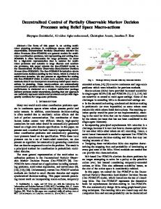
Fig. 1. Examples of partially observable PTAs (see Examples 1 and 2). 4

in Example 2. Checking this restriction can easily be done when exploring the discrete (digital clocks) semantics of the model – see below and Sec. 4. Semantics of POPTAs. We now formally define the semantics of a POPTA P, which is given in terms of an infinite-state POMDP. This extends the standard semantics of a PTA [27] (as an infinite MDP) with the same notion of observability we gave in Sec. 2 for POMDPs. The semantics, [[P]]T , is parameterised by a time domain T, giving the possible values taken by clocks. For the standard (dense-time) semantics of a POPTA, we take T = R. Later, when we discretise the model, we will re-use this definition, taking T = N. When referring to the “standard” semantics of P we will often drop the subscript R and write [[P]]. Definition 7 (POPTA semantics). Let P=(L, l, X , A, inv , enab, prob, r, OL , obs L ) be a POPTA. The semantics of P, with respect to the time domain T, is the POMDP [[P]]T =(S, s¯, A ∪ T, P, R, OL ×TX , obs) such that: – S = {(l, v) ∈ L×TX | v |= inv (l)} and s¯ = (l, 0); – for (l, v) ∈ S and a ∈ A ∪ T, we have P ((l, v), a) = µ if and only if: • (time transitions) a ∈ T, µ = δ(l,v+a) and v+t |= inv (l) for all 06t6a; • (action transition) a ∈ A, v |= enab(l, a) and for (l0 , v 0 ) ∈ S: P µ(l0 , v 0 ) = X⊆X ∧v0 =v[X:=0] prob(l, a)(X, l0 ) rL (l)·a if a ∈ T – for any (l, v) ∈ S and a ∈ A ∪ T, we have R((l, v), a) = rA (l, a) if a ∈ A – for any (l, v) ∈ S, we have obs(l, v) = (obs L (l), v). Example 1. Consider the POPTA in Fig. 1(a) with clocks x, y. Locations are grouped according to their observations, and we omit enabling conditions equal to true. We aim to maximise the probability of observing o5 . If locations were fully observable, we would leave l when x=y=1 and then, depending on whether the random choice resulted in a transition to l1 or l2 , wait 0 or 1 time units, respectively, before leaving the location. This would allow us to move immediately from l3 or l4 to l5 , meaning observation o5 is seen with probability 1. However, in the POPTA, we need to make the same choice in l1 and l2 since they yield the same observation. As a result, at most one of the transitions leaving locations l3 and l4 is enabled, and the probability of observing o5 is thus at most 0.5.

8

Norman, Parker, Zou

Digital clocks. Since the semantics of a POPTA (like for a PTA) is an infinitestate model, for algorithmic analysis, we first need to construct a finite representation. In this paper, we propose to use the digital clocks approach, generalising a technique already used for PTAs [20], which in turn adapts one for timed automata [16]. In short, this approach discretises a POPTA model by transforming its real-valued clocks to clocks taking values from a bounded set of integers. For clock x ∈ X , let kx denote the greatest constant to which x is compared in the clock constraints of POPTA P. If the value of x exceeds kx , its exact value will not affect the satisfaction of any invariants or enabling conditions, and thus not affect the behaviour of P. The digital clocks semantics, written [[P]]N , can be obtained from Defn. 7, taking T to be N instead of R. We also need to redefine the operation v+t, which now adds a delay t ∈ N to a clock valuation v ∈ NX : we say that v+t assigns the value min{v(x)+t, kx +1} to each clock x ∈ X . Under the restrictions on POPTAs described above, the digital semantics of a POPTA preserves the key properties required in this paper, namely optimal probabilities and expected cumulative rewards for reaching a specified observation. This is captured by the following theorem, which we prove in Appx. A. Theorem 1. If P is a closed, diagonal-free POPTA which resets only non-zero clocks, then, for any set of observations O of P and opt ∈ {min, max}, we have: opt opt opt Pr opt [[P]]R (F O) = Pr [[P]]N (F O) and E[[P]]R (F O) = E[[P]]N (F O).

The proof relies on showing probabilistic and expected reward values agree on the belief MDPs underlying the POMDPs representing the dense time and digital clocks semantics. This requires introducing the concept of a belief PTA for a POPTA (analogous to a belief MDP for a POMDP) and results for PTAs [20]. Example 2. The POPTA P in Fig. 1(b) demonstrates why our digital clocks approach (Thm. 1) is restricted to POPTAs which reset only non-zero clocks. We aim to minimise the expected reward accumulated before observing o3 (rewards are shown in Fig. 1(b) and are zero if omitted). If locations were fully observable, the minimum reward would be 0, achieved by leaving l immediately and then choosing a1 in l1 and a2 in l2 . However, if we leave l immediately, l1 and l2 are indistinguishable (we observe (o1,2 , (0)) when arriving in both), so we must choose the same action in these locations, and hence the expected reward is 0.5. Consider the strategy that waits ε ∈ (0, 1) before leaving l, accumulating a reward of ε. This is possible only in the dense-time semantics. We then observe either (o1,2 , (ε)) in l1 , or (o1,2 , (0)) in l2 . Thus, we see if x was reset, determine if we are in l1 or l2 , and take action a1 or a2 accordingly such that no further reward is accumulated before seeing o3 , for a total reward of ε. Since ε can be arbitrarily small, the minimum (infimum) expected reward for [[P]]R is 0. However, for the digital clocks semantics, we can only choose a delay of 0 or 1 in l. For the former, the expected reward is 0.5, as described above; for the latter, we can again pick a1 or a2 based on whether x was reset, for a total expected reward of 1. Hence the minimum expected reward for [[P]]N is 0.5, as opposed to 0 for [[P]]R .


4

9

Verification and Strategy Synthesis for POPTAs

We now present our approach for verification and strategy synthesis for POPTAs using the digital clock semantics given in the previous section. Property specification. First, we define a temporal logic for the formal specification of quantitative properties of POPTAs. This is based on a subset (we omit temporal operator nesting) of the logic presented in [27] for PTAs. Definition 8 (Properties). The syntax of our logic is given by the grammar: φ ::= P./p [ψ] R./q [ρ] ψ ::= α U6t α α U α α ::= true o ¬o ζ α ∧ α α ∨ α ρ ::= I=t C6t F α where o is an observation, ζ is a clock constraint, ./ ∈ {6, , >}, p ∈ Q∩[0, 1], q ∈ Q>0 and t ∈ N. A property φ is an instance of either the probabilistic operator P or the expected reward operator R. As for similar logics, P./p [ψ] means the probability of path formula ψ being satisfied is ./p, and R./q [ρ] the expected value of reward operator ρ is ./q. For the probabilistic operator, we allow time-bounded (α U6t α) and unbounded (α U α) until formulas, and adopt the usual equivalences such as F α ≡ true U α (“eventually α”). For the reward operator, we allow I=t (location reward at time instant t), C6t (reward accumulated until time t) and F α (the reward accumulated until α becomes true). Our propositional formulas (α) are Boolean combinations of observations and clock constraints. We omit nesting of P and R operators for two reasons: firstly, the digital clocks approach that we used to discretise time is not applicable to nested properties (see [20] for details); and secondly, it allows us to use a consistent property specification for either verification or strategy synthesis problems (the latter is considerably more difficult in the context of nested formulas [4]). Definition 9 (Property semantics). Let P be a POPTA with location observation function obs L and semantics [[P]]. We define satisfaction of a property φ from Defn. 8 with respect to a strategy σ ∈ Σ[[P]] as follows: [[P]], σ |= P./p [ ψ ] ⇐⇒ Pr σ[[P]] ({ω ∈ IPaths [[P]] | ω |= ψ}) ./ p [[P]], σ |= R ./q [ ρ ] ⇐⇒ Eσ[[P]] (rew (ρ)) ./ q Satisfaction of a path formula ψ by path ω, denoted ω |= ψ and the random variable rew (ρ) for a reward operator ρ are defined identically as for PTAs. Due to lack of space, we omit their formal definition here and refer the reader to [27]. For a propositional formula α and state s = (l, v) of [[P]], we have s |= o if and only if obs L (l)=o and s |= ζ if and only if v |= ζ. Boolean operators are standard. Verification and strategy synthesis. Given a POPTA P and property φ, we are interested in solving the dual problems of verification and strategy synthesis.

10

Norman, Parker, Zou

Definition 10 (Verification). The verification problem is: given a POPTA P and property φ, decide if [[P]],σ |= φ holds for all strategies σ∈Σ[[P]] . Definition 11 (Strategy synthesis). The strategy synthesis problem is: given POPTA P and property φ, find, if it exists, a strategy σ∈Σ[[P]] such that [[P]],σ |= φ. The verification and strategy synthesis problems for φ can be solved similarly, by computing optimal values for either probability or expected reward objectives: σ Pr min [[P]] (ψ) = inf σ∈Σ[[P]] Pr [[P]] (ψ) σ Pr max [[P]] (ψ) = supσ∈Σ[[P]] Pr [[P]] (ψ)

σ Emin [[P]] (ρ) = inf σ∈Σ[[P]] E[[P]] (ρ) σ Emax [[P]] (ρ) = supσ∈Σ[[P]] E[[P]] (ρ)

and, where required, also synthesising an optimal strategy. For example, verifying φ=P>p [ ψ ] requires computation of Pr min [[P]] (ψ) since φ is satisfied by all strategies if and only if Pr min (ψ)>p. Dually, consider synthesising a strategy for which [[P]] φ0 =P6p [ ψ ] holds. Such a strategy exists if and only if Pr min [[P]] (ψ)6p and, if it does, we can use the optimal strategy that achieves the minimum value. A common practice in probabilistic verification to simply query the optimal values directly, using numerical properties such as Pmin=? [ ψ ] and R max=? [ ρ ]. As mentioned earlier, when solving POPTAs (or POMDPs), we may only be able to under- and over-approximate optimal values, which requires adapting the processes sketched above. For example, if we have determined lower and upper ] [ bounds p[ 6 Pr min [[P]] (ψ) 6 p . We can verify that φ=P>p [ ψ ] holds if p > p or ascertain that φ does not hold if p > p] . But, if p[ < p < p] , we need to refine our approximation to produce tighter bounds. An analogous process can be followed for the case of strategy synthesis. The remainder of this section therefore focuses on how to (approximately) compute optimal values and strategies for POPTAs. Numerical computation algorithms. Approximate numerical computation of either optimal probabilities or expected reward values on a POPTA P is performed with the sequence of steps given below, each of which is described in more detail subsequently. We compute both an under- and an over-approximation. For the former, we also generate a strategy which achieves this value. (A) We modify POPTA P, reducing the problem to computing optimal values for a probabilistic reachability or expected cumulative reward property [27]; (B) We apply the digital clocks discretisation of Sec. 3 to reduce the infinite-state semantics [[P]]R of P to a finite-state POMDP [[P]]N ; (C) We build and solve a finite abstraction of the (infinite-state) belief MDP B([[P]]N ) of the POMDP from (B), yielding an over-approximation; (D) We synthesise and analyse a strategy for [[P]]N , giving an under-approximation; (E) If required, we refine the abstraction’s precision and repeat (C) and (D). (A) Property reduction. As discussed in [27] (for PTAs), checking P or R properties of the logic of Defn. 8 can always be reduced to checking either a probabilistic reachability (P./p [F α]) or expected cumulative reward (R./q [F α]) property on a modified model. For example, time-bounded probabilistic reachability


11

(P./p [F6t α]) can be transformed into probabilistic reachability (P./p [F (α∧y6t)]) where y is a new clock added to the model. We refer to [27] for full details. (B) Digital clocks. We showed in Sec. 3 that, assuming certain simple restrictions on the POPTA P, we can construct a finite POMDP [[P]]N representing P by treating clocks as bounded integer variables. The translation itself is relatively straightforward, involving a syntactic translation of the PTA (to convert clocks), followed by a systematic exploration of its finite state space. At this point, we also check satisfaction of the restrictions on POPTAs described in Sec. 3. (C) Over-approximation. We now solve the finite POMDP [[P]]N . For simplicity, here and below, we describe the case of maximum reachability probabilities (the other cases are very similar) and thus need to compute Pr max [[P]]N (F O). We first compute an over-approximation, i.e. an upper bound on the maximum probability. This is computed from an approximate solution to the belief MDP B([[P]]N ), whose construction we outlined in Sec. 2. This MDP has a continuous state space: the set of beliefs Dist(S), where S is the state space of [[P]]N . To approximate its solution, we adopt the approach of [29] which computes values for a finite set of representative beliefs G whose convex hull is Dist(S). Value iteration is applied to the belief MDP, using the computed values for beliefs in G and interpolating to get values for those not in G. The resulting values give the required upper bound. We use [29] as it works with unbounded (infinite horizon) and undiscounted properties. There are many other similar approaches [28], but these are formulated for discounted or finite-horizon properties. The representative beliefsPcan be chosen in a variety of ways. We follow [23], |S| 1 v | v ∈ N|S| ∧ i=1 v(i)=M }, i.e. a uniform grid with resolution where G = { M M . A benefit is that interpolation is very efficient, using a process called triangulation [13]. A downside is that the grid size is exponential M . (D) Under-approximation. Since it is preferable to have two-sided bounds, we also compute an under-approximation: here, a lower bound on Pr max [[P]]N (F O). To do so, we first synthesise a finite-memory strategy σ ∗ for [[P]]N (which is often a required output anyway). The choices of this strategy are built by stepping through the belief MDP and, for the current belief, choosing an action that achieves the values returned by value iteration in (C) above – see for example [28]. We then compute, by building and solving the finite Markov chain induced by ∗ [[P]]N and σ ∗ , the value Pr σ[[P]]N (F O) which is a lower bound for Pr max [[P]]N (F O). (E) Refinement. Finally, although no a priori bound can be given on the error between the generated under- and over-approximations (recall that the basic problem is undecidable), asymptotic convergence of the grid based approach is guaranteed [29]. In practice, if the computed approximations do not suffice to verify the required property (or, for strategy synthesis, σ ∗ does not satisfy the property), then we increase the grid resolution M and repeat steps (C) and (D).

12

5

Norman, Parker, Zou

Implementation and Case Studies

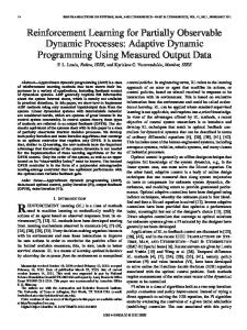
We have built a prototype tool for verification and strategy synthesis of POPTAs and POMDPs as an extension of PRISM [19]. We extended the existing modelling language for PTAs, to allow model variables to be specified as observable or hidden. The tool performs the steps outlined in Sec. 4, computing a pair of bounds for a given property and synthesising a corresponding strategy. We focus on POPTAs, but the tool can also analyse POMDPs directly. The software, details of all case studies, parameters and properties are available online at: http://www.prismmodelchecker.org/files/formats15poptas/ We have developed three case studies to evaluate the tool and techniques, discussed in more detail below. In each case, nondeterminism, probability, real-time behaviour and partial observability are all essential aspects required for analysis. The NRL pump. The NRL (Naval Research Laboratory) pump [17] is designed to provide reliable and secure communication over networks of nodes with ‘high’ and ‘low’ security levels. It prevents a covert channel leaking information from ‘high’ to ‘low’ through the timing of messages and acknowledgements. Communication is buffered and probabilistic delays are added to acknowledgements from ‘high’ in such a way that the potential for information leakage is minimised, while maintaining network performance. A PTA model is considered in [21]. We model the pump as a POPTA using a hidden variable for a secret value z ∈ {0, 1} (initially set uniformly at random) which ‘high’ tries to covertly communicate to ‘low’. This communication is attempted by adding a delay of h0 or h1 , depending on the value of z, whenever sending an acknowledgement to ‘low’. In the model, ‘low’ sends N messages to ‘high’ and tries to guess z based on the time taken for its messages to be acknowledged. We consider the maximum probability ‘low’ can (either eventually or within some time frame) correctly guess z. We also study the expected time to send all messages and acknowledgements. These properties measure the security and performance aspects of the pump. Results are presented in Fig. 2 varying h1 and N (we fix h0 =2). They show that increasing either the difference between h0 and h1 (i.e., increasing h1 ) or the number N of messages sent improve the chance of ‘low’ correctly guessing the secret z, at the cost of a decrease in network performance. On the other hand, when h0 =h1 , however many messages are sent, ‘low’, as expected, learns nothing of the value being sent and at best can guess correctly with probability 0.5. Task-graph scheduler. Secondly, we consider a task-graph scheduling problem adapted from [7], where the goal is to minimise the time or energy consumption required to evaluate an arithmetic expression on multiple processors with different speeds and energy consumption. We extend both the basic model of [7] and the extension from [27] which uses PTAs to model probabilistic task execution times. A new ‘low power’ state to one processor, allowing it to save energy when not in use, but which incurs a delay when waking up to execute a new task. This state is entered with probability sleep after each task is completed. We assume that the scheduler cannot observe whether the processor enters this lower

1

expected time to transmit

max. prob guess correctly


0.8

0.6

0.4 20

400 300 200 100 0 20 20

20 15

10 N

10 0 0

(a)

1

15

10

5 h

13

N

10 0 0

5 h

1

(b)

Fig. 2. Analysing security/performance of the NRL pump: (a) Maximum probability of covert channel success; (b) Maximum expected transmission time.

power state, and hence the model is a POPTA. We generate optimal schedulers (minimising expected execution time or energy usage) using strategy synthesis. Non-repudiation protocol. Our third case study is a non-repudiation protocol for information transfer due to Markowitch & Roggeman [25]. It is designed to allow an originator O to send information to a recipient R while guaranteeing non-repudiation, that is, neither party can deny having participated in the information transfer. The initialisation step of the protocol requires O to randomly select an integer N in the range 1, . . . , K that is never revealed to R during execution. In previous analyses [22,27], modelling this step was not possible since no notion of (non-)observability was used. We resolve this by building a POPTA model of the protocol including this step, thus matching Markowitch & Roggeman’s original specification. In particular, we include a hidden variable to store the random value N . We build two models: a basic one, where R’s only malicious behaviour corresponds to stopping early; and a second, more complex model, where R has access to a decoder. We compute the maximum probability that R gains an unfair advantage (gains the information from O while being able to deny participating). Our results (see Table 1) show that, for the basic model, this probability equals 1/K and R is more powerful in the complex model. Experimental results. Table 1 summarises a representative set of experimental results from the analysis of our three case studies. All were run on a 2.8 GHz PC with 8GB RAM. The table shows the parameters used for each model (see the web page cited above for details), the property analysed and various statistics from the analysis: the size of the POMDP obtained through the digital clocks semantics; number of observations; number of hidden values (i.e., the maximum number of states with the same observation); the grid size (resolution M and total number of points); the time taken; and the results obtained. For comparison, in the rightmost column, we show what result is obtained if the POPTA is treated as a PTA (by making everything observable). On the whole, we find that the performance of our prototype is good, especially considering the complexity of the POMDP solution methods and the

14

Norman, Parker, Zou Case study (parameters)

pump (h1 N ) pump (h1 N D) scheduler basic (sleep) scheduler basic (sleep) scheduler prob (sleep) scheduler prob (sleep) nrp basic (K) nrp complex (K)

16 2 16 2 16 16 8 4 50 8 4 50 16 8 50 16 8 100 0.25 0.5 0.75 0.25 0.5 0.75 0.25 0.5 0.75 0.25 0.5 0.75 4 4 8 8 4 4 8 8

Verification/strategy synthesis of POPTA States Num. Num. Res. Grid Time Result ([[P]]N ) obs. hidd. (M ) points (s) (bounds) 243 145 3 2 342 0.7 [0.940, 0.992] Pmax=? [F guess] 243 145 3 40 4,845 4.0 [0.940, 0.941] 1,559 803 3 2 2,316 16.8 [0.999, 0.999] 12,167 7,079 3 2 17,256 11.0 [0.753, 0.808] 12,167 7,079 3 12 68,201 36.2 [0.763, 0.764] Pmax=? [F6D guess] 26,019 13,909 3 2 38,130 52.8 [0.501, 0.501] 59,287 31,743 3 2 86,832 284.8 [0.531, 0.532] 5,002 3,557 2 2 6,447 3.2 [14.69, 14.69] Rmin=? [F done] 5,002 3,557 2 2 6,447 3.1 [17.0, 17.0] (exec. time) 5,002 3,557 2 4 9,337 3.1 [19.25, 19.25] 5,002 3,557 2 4 9,337 3.1 [1.335, 1.335] Rmin=? [F done] 5,002 3,557 2 2 6,447 3.1 [1.270, 1.270] (energy cons.) 5,002 3,557 2 2 6,447 3.2 [1.204, 1.204] 6,987 5,381 2 2 8,593 5.8 [15.00, 15.00] Rmin=? [F done] 6,987 5,381 2 2 8,593 5.8 [17.27, 17.27] (exec. time) 6,987 5,381 2 4 11,805 5.0 [19.52, 19.52] 6,987 5,381 2 4 11,805 5.3 [1.335, 1.335] Rmin=? [F done] 6,987 5,381 2 2 8,593 5.0 [1.269, 1.269] (energy cons.) 6,987 5,381 2 2 8,593 5.8 [1.204, 1.204] 365 194 5 8 5,734 0.8 [0.25, 0.281] 365 194 5 24 79,278 5.9 [0.25, 0.25] Pmax=? [F unfair ] 1,273 398 9 4 23,435 4.8 [0.125, 0.375] 1,273 398 9 8 318,312 304.6 [0.125, 0.237] 1,501 718 5 4 7,480 2.1 [0.438, 0.519] 1,501 718 5 12 72,748 14.8 [0.438, 0.438] Pmax=? [F unfair ] 5,113 1,438 9 2 16,117 6.1 [0.344, 0.625] 5,113 1,438 9 4 103,939 47.1 [0.344, 0.520] Property

PTA result 1.0 1.0 1.0 1.0 1.0 1.0 1.0 14.44 16.5 18.5 1.237 1.186 1.155 14.75 16.77 18.77 1.3 1.185 1.155 1.0 1.0 1.0 1.0 1.0 1.0 1.0 1.0

Table 1. Experimental results from verification/strategy synthesis of POPTAs.

fact that we use a relatively simple grid mechanism. We are able to analyse POPTAs whose integer semantics yields POMDPs of up to 60,000 states, with experiments usually taking just a few seconds and, at worst, 5-6 minutes. These are, of course, smaller than the standard PTA (or MDP) models that can be verified, but we were still able to obtain useful results for several case studies. The values in the rightmost column of Table 1 illustrate that the results obtained with POPTAs would not have been possible using a PTA model, i.e., where all states of the model are observable. For the pump example, the PTA gives probability 1 of guessing correctly (‘low’ can simply read the value of the secret). For the scheduler example, the PTA model gives a scheduler with better time/energy consumption but that cannot be implemented in practice since the power state is not visible. For the nrp models, the PTA gives probability 1 of unfairness as the recipient can read the random value the originator selects. Another positive aspect is that, in many cases, the bounds generated are very close (or even equal, in which case the results are exact). For the pump and scheduler case studies, we included results for the smallest grid resolution M required to ensure the difference between the bounds is at most 0.001. In many cases, this is achieved with relatively small values (for the scheduler example, in particular, M is at most 4). For nrp models, we were unable to do this when K=8 and instead include the results for the largest grid resolution for which POMDP solution was possible: higher values could not be handled within the memory


15

constraints of our test machine. We anticipate being able to improve this in the future by adapting more advanced approximation methods for POMDPs [28].

6

Conclusions

We have proposed novel methods for verification and control of partially observable probabilistic timed automata, using a temporal logic for probabilistic, real-time properties and reward measures. We developed techniques based on a digital clocks discretisation and a belief space approximation, then implemented them in a tool and demonstrated their effectiveness on several case studies. Future directions include more efficient approximation schemes, zone-based implementations and development of the theory for unobservable clocks. Allowing unobservable clocks, as mentioned previously, will require moving to partially observable stochastic games and restricting the class of strategies. Acknowledgments. This work was partly supported by the EPSRC grant “Automated Game-Theoretic Verification of Security Systems” (EP/K038575/1). We also grateful acknowledge support from Google Summer of Code 2014.

References 1. de Alfaro, L.: The verification of probabilistic systems under memoryless partialinformation policies is hard. In: Proc. PROBMIV’99. pp. 19–32 (1999) 2. Alur, R., Dill, D.: A theory of timed automata. Theoretical Computer Science 126, 183–235 (1994) 3. Baier, C., Bertrand, N., Gr¨ oßer, M.: On decision problems for probabilistic B¨ uchi automata. In: Proc. FOSSACS’08. LNCS, vol. 4962, pp. 287–301. Springer (2008) 4. Baier, C., Gr¨ oßer, M., Leucker, M., Bollig, B., Ciesinski, F.: Controller synthesis for probabilistic systems. In: Proc. TCS’06. pp. 493–506. Kluwer (2004) 5. Behrmann, G. et al.: Minimum-cost reachability for linearly priced timed automata. In: Proc. HSCC’01. LNCS, vol. 2034, pp. 147–162. Springer (2001) 6. Bouyer, P., D’Souza, D., Madhusudan, P., Petit, A.: Timed control with partial observability. In: Proc. CAV’03. LNCS, vol. 2725, pp. 180–192 (2003) 7. Bouyer, P., Fahrenberg, U., Larsen, K., Markey, N.: Quantitative analysis of realtime systems using priced timed automata. Comm. of the ACM 54(9), 78–87 (2011) 8. Cassandra, A.: A survey of POMDP applications (1998), http://pomdp.org/ pomdp/papers/applications.pdf, presented at the AAAI Fall Symposium, 1998 9. Cassez, F., David, A., Larsen, K., Lime, D., Raskin, J.F.: Timed control with observation based and stuttering invariant strategies. In: Proc. ATVA’07. LNCS, vol. 4762, pp. 192–206 (2007) 10. Cern´ y, P., Chatterjee, K., Henzinger, T., Radhakrishna, A., Singh, R.: Quantitative synthesis for concurrent programs. In: Proc. CAV’11. LNCS, vol. 6806, pp. 243– 259. Springer (2011) 11. Chatterjee, K., Chmelik, M., Tracol, M.: What is decidable about partially observable Markov decision processes with omega-regular objectives. In: CSL’13. LIPIcs, vol. 23, pp. 165–180. Schloss Dagstuhl–Leibniz-Zentrum fuer Informatik (2013)

16

Norman, Parker, Zou

12. Chatterjee, K., Doyen, L.: Partial-observation stochastic games: How to win when belief fails. ACM Transactions on Computational Logic 15(2) (2014) 13. Eaves, B.: A course in triangulations for solving equations with deformations. Springer (1984) 14. Finkbeiner, B., Peter, H.: Template-based controller synthesis for timed systems. In: Proc. TACAS’12. LNCS, vol. 7214, pp. 392–406 (2012) 15. Giro, S., Rabe, M.: Verification of partial-information probabilistic systems using counterexample-guided refinements. In: Proc. ATVA’12. LNCS, vol. 7561, pp. 333– 348. Springer (2012) 16. Henzinger, T., Manna, Z., Pnueli, A.: What good are digital clocks? In: Proc. ICALP’92. LNCS, vol. 623, pp. 545–558. Springer (1992) 17. Kang, M., Moore, A., Moskowitz, I.: Design and assurance strategy for the NRL pump. Computer 31(4), 56–64 (1998) 18. Kemeny, J., Snell, J., Knapp, A.: Denumerable Markov Chains (1976) 19. Kwiatkowska, M., Norman, G., Parker, D.: PRISM 4.0: Verification of probabilistic real-time systems. In: Proc. CAV’11. LNCS, vol. 6806, pp. 585–591. Springer (2011) 20. Kwiatkowska, M., Norman, G., Parker, D., Sproston, J.: Performance analysis of probabilistic timed automata using digital clocks. FMSD 29, 33–78 (2006) 21. Lanotte, R., Maggiolo-Schettini, A., Tini, S., Troina, A., Tronci, E.: Automatic analysis of the NRL pump. ENTCS 99, 245–266 (2004) 22. Lanotte, R., Maggiolo-Schettini, A., Troina, A.: Automatic analysis of a nonrepudiation protocol. In: Proc. QAPL’04. ENTCS, vol. 112, pp. 113–129 (2005) 23. Lovejoy, W.: Computationally feasible bounds for partially observed Markov decision processes. Operations Research 39(1), 162–175 (1991) 24. Madani, O., Hanks, S., Condon, A.: On the undecidability of probabilistic planning and related stochastic optimization problems. Artif. Intell. 147(1–2), 5–34 (2003) 25. Markowitch, O., Roggeman, Y.: Probabilistic non-repudiation without trusted third party. In: Proc. Workshop on Security in Communication Networks (1999) 26. Norman, G., Parker, D., Zou, X.: Verification and control of partially observable probabilistic real-time systems. In: Proc. FORMATS’15. LNCS, Springer (2015), to appear 27. Norman, G., Parker, D., Sproston, J.: Model checking for probabilistic timed automata. FMSD 43(2), 164–190 (2013) 28. Shani, G., Pineau, J., Kaplow, R.: A survey of point-based POMDP solvers. Autonomous Agents and Multi-Agent Systems 27(1), 1–51 (2013) 29. Yu, H.: Approximate Solution Methods for Partially Observable Markov and SemiMarkov Decision Processes. Ph.D. thesis, MIT (2006)


A

17

Proof of Thm. 1

As discussed in Sec. 3, we restrict our attention to POPTAs which reset only nonzero clocks. Given any clock valuations v, v 0 and distinct sets of clocks X, Y such that v(x)>0 for any x ∈ X ∪ Y we have that v[X:=0] = v 0 implies v[Y :=0] 6= v 0 . Therefore, under this restriction, for a time domain T and POPTA P, if there a exists a transition (l, v) to (l0 , v 0 ) in [[P]]T , then there is a unique set of clocks which are reset when this transition is taken and we define this set as follows. Definition 12. For any clock valuations v, v 0 ∈ TX we define the set of clocks X[v 7→ v 0 ] as follows: X[v7→v0 ] = {x ∈ X | v(x)>0 ∧ v 0 (x)=0}. Using Defn. 12, the transition function of [[P]]T is such that, for any (l, v) ∈ S and a ∈ A, we have P ((l, v), a)=µ if and only if v |= enab(l, a) and for (l0 , v 0 ) ∈ S: prob(l, a)(X[v7→v0 ] , l0 ) if v[X[v7→v0 ] :=0] = v 0 µ(l0 , v 0 ) = 0 otherwise. Before we present the proof of Thm. 1, we require the concept of a belief PTA. Definition 13. Given a POPTA P=(L, l, X , A, inv , enab, prob, r, OL , obs L ), the belief PTA is given by B(P) = (Dist obs L , δl , X , A, inv B , enab B , prob B , rB ) where – Dist obs L ⊆ Dist(L) where λ ∈ Dist obs L if and only if for any l, l0 ∈ L such that λ(l)>0 and λ(l0 )>0 we have obs L (l) = obs L (l0 ); – the invariant inv B : Dist obs L →CC (X ) and enabling conditions enab B : Dist obs L ×A → CC (X ) are such that for λ ∈ Dist obs L and a ∈ A we have inv B (λ)=inv (l) and enab B (λ, a)=enab(l, a) where l ∈ L is such that λ(l)>0; – the probabilistic transition function prob B : Dist obs L ×A → Dist(2X ×Dist obs L ) is such that for any λ, λ0 ∈ Dist obs L , a ∈ A and X ⊆ X we have: ! P P P B 0 0 prob (λ, a)(λ , X) = λ(l) · prob(l, a)(l , X) l∈L

o∈O∧λa,o,X =λ0 l0 ∈L∧obs L (l0 )=o

where for any l0 ∈ L we have  P 0 l∈L prob(l,a)(l ,X)·λ(l) P P if obs L (l0 )=o a,o,X 0 0 λ(l)· λ (l ) = l∈L l0 ∈L∧obs L (l0 )=o prob(l,a)(l ,X)  0 otherwise; B B – the reward structure rB =(rL , rA ) is such that P P B B rL (λ) = l∈L λ(l)·rL (l) and rA (λ, a) = l∈L λ(l) · r(l, a) .

For the above to be well defined we require the conditions of the invariant and observation function given in Defn. 6. For any λ ∈ Dist obs L we let oλ be the unique observation such that obs L (l) = oλ and λ(l) > 0 for some l ∈ L. Next we introduce the semantics of a PTA which, similarly to Defn. 7, is parameterised by a time domain T.

18

Norman, Parker, Zou

Definition 14 (PTA semantics). Let P = (L, l, X , A, inv , enab, prob, r) be a probabilistic timed automaton. The semantics of P with respect to the time domain T is the MDP [[P]]T = (S, s¯, A ∪ T, P, R) such that: – S = {(l, v) ∈ L × TX | v |= inv (l)} and s¯ = (l, 0); – for any (l, v) ∈ S and a ∈ A ∪ T, we have P ((l, v), a) = µ if and only if one of the following conditions hold: • (time transitions) a ∈ T, µ = δ(l,v+a) and v+a |= inv (l) for all 06t0 6a; • (action transition) a ∈ A, v |= enab(l, a) and for (l0 , v 0 ) ∈ S: P µ(l0 , v 0 ) = X⊆X ∧v0 =v[X:=0] prob(l, a)(X, l0 ) rL (l)·a if a ∈ T – for any (l, v) ∈ S and a ∈ A ∪ T: R((l, v), a) = rA (l, a) if a ∈ A. We now show that for a POPTA P, the semantics of its belief PTA is equivalent to the belief MDP of the semantics of P. Proposition 1. For any POPTA P which resets only non-zero clocks, time domain T we have that the MDPs [[B(P)]]T and B([[P]]T ) are equivalent. Proof. Consider any POPTA P = (L, l, X , A, inv , enab, prob, r, OL , obs L ) which resets only non-zero clocks and time domain T. To show the MDPs [[B(P)]]T and B([[P]]T ) are equivalent we will first give a direct correspondence between their state spaces and then show that under this correspondence both the transition and reward functions are equivalent. Considering the belief MDP B([[P]]T ) and using the fact that obs(l, v) = (obs L (l), v), for any belief states b, b0 and action a we have P B (b, a)(b0 ) equals   X X X 0 b(l, v) ·  P ((l, v), a)(l , vo ) (o,vo )∈O×TX (l,v)∈S ba,(o,vo ) =b0

l0 ∈L∧obs L (l0 )=o

where for any belief b, action a, observation (o, vo ) and state (l0 , v 0 ), we have ba,(o,vo ) (l0 , v 0 ) equals  P 0 0 (l,v)∈S P ((l,v),a)(l ,v )·b(l,v) P P if obs L (l0 )=o and v 0 =vo 00 0 b(l,v)· (1) (l,v)∈S l00 ∈L∧obs L (l00 )=o P ((l,v),a)(l ,v )  0 otherwise P and RB (b, a) = (l,v)∈S R((l, v), a) · b(l, v). Furthermore, by Defn. 7 and since in P only non-zero clocks are reset, if a ∈ A: prob(l, a)(X[v7→v0 ] , l0 ) if v[X[v7→v0 ] :=0] = v 0 0 0 P ((l, v), a)(l , v ) = (2) 0 otherwise while if a ∈ T: P ((l, v), a)(l0 , v 0 ) =

1 if l0 =l and v 0 = v+a 0 otherwise.

(3)


19

We see that ba,(o,vo ) (l0 , v 0 ) is zero if v 0 6= vo , and therefore we can write the belief as (λ, vo ) where λ ∈ Dist(L) and λ(l) = ba,(o,vo ) (l, vo ) for all l ∈ L. In addition, for any l0 ∈ L, if λ(l0 )>0, then obs L (l0 )=o. Since the initial belief ¯b can be written as (δl , 0) and we assume obs L (l) 6= obs L (l) for any l 6= l ∈ L, it follows that we can write each belief b of B([[P]]T ) as a tuple (λ, v) ∈ Dist(L) × TX such that for any l, l0 ∈ L, if λ(l)>0 and λ(l0 )>0, then obs L (l)=obs L (l0 ). Hence, we have shown that the states of B([[P]]T ) are equivalent to the states of [[B(P)]]T . We now use this representation for the states of B([[P]]T ) to rewrite the above equations for the transition and reward function of the belief MDP B([[P]]T ). We have the following two cases to consider. – For any belief states (λ, v) and (λ0 , v 0 ) and action a ∈ A:  X

X

P B ((λ, v), a)(λ0 , v 0 ) =

o∈OL l∈L 0 λa,(o,v ) =λ0

X

X

o∈OL l∈L 0 λa,(o,v ) =λ0

X l∈L

l0 ∈L O(l0 )=o

  X prob(l, a)(X[v7→v0 ] , l0 ) λ(l) ·   

by (2)

0

l ∈L O(l0 )=o



 =

  X P ((l, v), a)(l0 , v 0 ) λ(l) ·    

 =



X

 λ(l) ·  

X

o∈OL l0 ∈L 0 0 λa,(o,v ) =λ0 O(l )=o

 prob(l, a)(X[v7→v0 ] , l0 ) 

rearranging

where for any l0 ∈ L:  P P ((l,v),a)(l0 ,v 0 )·λ(l) P Pl∈L if obs L (l0 ) = o 0 a,(o,v ) 0 00 0 λ(l)· 00 λ (l ) = l∈L l ∈L∧obs L (l00 )=o P ((l,v),a)(l ,v )  0 otherwise  P 0 prob(l,a)(X ,l )·λ(l) 0 [v7→v ] l∈L P P if obs L (l0 )=o 0 = by (2) l∈L λ(l)· l00 ∈L∧obs L (l00 )=o prob(l,a)(X[v7→v 0 ] ,l )  0 otherwise = λa,o,X[v7→v0 ]

by Defn. 13.

Using this result together with Defn. 13 and Defn. 14 it follows that the transition functions of B([[P]]T ) and [[B(P)]]T are equivalentP in the case. Considering the reward functions, we have RB ((λ, v), a) = l∈L rA (l, a)·λ(l) which, again from Defn. 13 and Defn. 14, shows that the reward functions of B([[P]]T ) and [[B(P)]]T are equivalent. – For any belief states (λ, v) and (λ0 , v 0 ) and time duration t ∈ T: B

0

0

P ((λ, v), t)(λ , v ) =

P

l∈L

0

λ(l) · P ((l, v), a)(l, v 0 ) if λt,(oλ ,v ) =λ0 0 otherwise

20

Norman, Parker, Zou

where for any l0 ∈ L: ( λ

t,(oλ ,v 0 )

0

(l ) =

0

=

0 P λ(l ) l∈L λ(l)

if v 0 = v+t otherwise

0

λ(l ) if v 0 = v+t 0 otherwise

since λ is a distribution. 0

Substituting this expression for λt,(oλ ,v ) into that of P B ((λ, v), t) we have: P B ((λ, v), t)(λ0 , v 0 ) P P 0 0 0 0 λ(l) · 0 ∈L P ((l, v), a)(l , v ) if λ=λ and v = v+t l l∈L = 0 otherwise P 0 0 l∈L λ(l) if λ=λ and v = v+t = by (3) 0 otherwise 1 if λ=λ0 and v 0 = v+t = since λ is a distribution 0 otherwise which from Defn. 13 and Defn. 14 shows the transition functions of B([[P]]T ) B and P [[B(P)]]T are equivalent. For the reward function, we have R ((λ, v), t) = l∈L (rL (l)·t)·λ(l) and from Defn. 13 and Defn. 14 this implies that the reward functions of B([[P]]T ) and [[B(P)]]T again are equivalent. Since these are the only cases to consider, both the transition and reward functions of B([[P]]T ) and [[B(P)]]T are equivalent completing the proof. t u We are now in a position to present the proof of Thm. 1. Proof (of Thm. 1). Consider any closed diagonal-free POPTA P which resets only non-zero clocks and set of observations O of P. Since the PTA B(P) is closed and diagonal-free, using results presented in [20], we have that: opt opt opt Pr opt [[B(P)]]R (F TO ) = Pr [[B(P)]]N (F TO ) and E[[B(P)]]R (F TO ) = E[[B(P)]]N (F TO ) (4)

where opt ∈ {min, max} and To = {(l, v) | obs(l) ∈ O}. Note that, although [20] considers only PTAs with finite locations, the corresponding proofs do not require this fact, and hence the results carry over to B(P) which has an uncountable number of locations. Due to the equivalence between a POMDP and its belief MDP we have: opt opt opt Pr opt [[P]]T (F O) = Pr B([[P]]T ) (F TO ) and E[[P]]T (F O) = EB([[P]]T ) (F TO ).

(5)

Using Proposition 1 and since P resets only non-zero clocks we have [[B(P)]]T = B([[P]]T ). Combining this with (4) and (5) the theorem follows. t u

B

Construction of the Belief MDP

For the convenience of the reviewers, below we include, for a given POMDP M, the construction of the corresponding belief MDP B(M).


21

First, let us suppose we are in a belief state b, perform action a and observe o. Based on this new information we move to a new belief state ba,o using the observation function of M. Let us now construct this new belief state. First, by construction, we have for any s0 ∈ S: ba,o (s0 ) = Pr[ s0 | o, a, b ] Pr[ s0 , o, a, b ] Pr[ o, a, b ]   Pr[ s0 , a, b ] if obs(s0 ) = o = Pr[ o, a, b ]  0 otherwise

by definition of conditional probabilities

=

by definition of obs.

Now considering the numerator in the first case, since the value of s0 is dependent on the other values: Pr[ s0 , a, b ] = Pr[ s0 | a, b ] · Pr[ a, b ] = Pr[ s0 | a, b ] · 1 P = Pr[ s0 | a, s ] · b(s) Ps∈S 0 = s∈S P (s, a)(s ) · b(s)

since b and a are fixed definition of b definition of P .

For the denominator since o is dependent on b and a we have: Pr[ o, a, b ] = Pr[ o | a, b ] · Pr[ a, b ] = Pr[ o | a, b ] · 1 P = s∈S Pr[ o | a, s ] · b(s) P P 0 0 = s∈S s0 ∈S Pr[ o | s , a ] · P (s, a)(s ) · b(s) P P 0 = P (s, a)(s ) · b(s) 0 0 s∈S s ∈S∧obs(s )=o Combining these results (and rearranging) we have: P ( P (s,a)(s0 )·b(s) ba,o (s0 ) =

P

s∈S

since b and a are fixed by definition of b by definition of P by definition of obs.

s∈S P b(s)·( s00 ∈S∧obs(s00 )=o P (s,a)(s00 ))

0

if obs(s0 )=o otherwise.

Now using this we can define the probabilistic transition function of the belief MDP B(M). Suppose we are in a belief state b and we perform action a. Now the probability we move to belief b0 is given by: P 0 PTB (b, a)(b0 ) = Pr[ b0 | a, b ] = o∈O Pr[ b | o, a, b ] · Pr[ o | a, b ] . The first term in the summation (Pr[ b0 | o, a, b ]) is the probability of being in belief b0 after being in belief b, performing action a and observing o. Therefore by definition of ba,o , this probability will equal 1 if b0 equals ba,o and 0 otherwise. For the second term, as in the derivation of the denominator above, we have: P P 0 Pr[ o | a, b ] = s∈S b(s) · s0 ∈S∧obs(s0 )=o P (s, a)(s )

22

Norman, Parker, Zou

This completes the construction of the transition function of the belief MDP. It remains to construct the reward function RB of the belief MDP. In this case, we just have to take the expectation of the reward with respect to the current belief, i.e. for any action a and belief state b: P RB (b, a) = s∈S R(s, a) · b(s) . The optimal values for the belief MDP equal those for the POMDP, e.g. we have: max max max Pr max M (F O) = Pr B(M) (F TO ) and EM (F O) = EB(M) (F TO )

where TO = {b ∈ Dist(S) | ∀s ∈ S. (b(s)>0 → obs(s) ∈ O)}.