Jan 26, 2004 - in numerical simulations of multipacting, a multipacting test code ..... ing a single surface only, i.e. electrons return to the same point from which.
Veri cation of a Multipacting Computer Code and Analysis of an RF Test Cavity
Diploma Thesis
Registration number 183194
26.01.2004
CERN-THESIS-2004-008
submitted by Clemens Schulz
Technische Universit at Berlin Fakult at IV Elektrotechnik und Informatik Fachgebiet Theoretische Elektrotechnik supervising Professor: H. Henke (TU-Berlin) supervising Assistant: F. Gerigk (CERN)
January 2004
1
Abstract
A design study has been carried out at the European Organization for Nuclear Research (CERN), to de ne layout and parameters of a future neutrino
factory [2], [18]. The reference scheme of this neutrino factory incorporates a muon cooling channel, which partly consists of 88 MHz accelerating cavities [15]. In order to reveal possible technical diÆculties in achieving the desired gradient of 4 MV/m, a 88 MHz test cavity has been constructed. The present work aimed to test this cavity for multipacting discharges. For this purpose CERN has acquired the multipacting simulation code MultP [25],[24]. In a rst step two known examples of multipacting were analysed, to check the functionality of the code. The tests revealed that MultP lacked some means to predict multipacting. Moreover, MultP partly produced erroneous results. In order to nd their origin and to gain a deeper understanding in numerical simulations of multipacting, a multipacting test code has been programmed for those two examples. The test code was then succesfully used to nd the origin of the errors. Two new functions were eventually implemented into MultP: the electron counter and the distance function. Thus, the analysis became more reliable and easier to perform. Finally, a multipacting analysis of the test cavity was carried out. Two possible barriers have been discovered. The rst barrier is between 180 kV and 200 kV gap voltage, and the second is at 130 kV gap voltage. They are both far below the operating level of 4 MV. An experimental veri cation of these multipacting levels shall be done at CERN.
Zusammenfassung
Im Rahmen einer Design-Studie eines Myon-Cooling Kanals fur eine zukunftige Neutrinoquelle [2], [18] wurde am europaischen Teilchenforschungszentrum, CERN, zu Testzwecken eine 88 MHz Beschleunigerzelle aufgebaut. Diese sollte durch Simulation mit einem Computerprogramm auf das Auftreten resonanter Hochfrequenzentladungen (Multipacting) untersucht werden. Zu diesem Zweck stand dem CERN das Multipacting-Simulationsprogramm MultP [25],[24] zur Verfugung. Zunachst wurden die Fahigkeiten von MultP anhand zweier einfacher Beispielfalle, deren Losungen bekannt waren, gepruft. Es stellte sich heraus, dass es MultP an einigen Analysemoglichkeiten mangelte und die Resultate au�erdem fehlerbehaftet waren. Um die Ursache der Fehler in MultP zu ergrunden, und um die Schwierigkeiten einer numerischen Analyse besser zu verstehen, wurde fur die beiden Beispielfalle ein einfaches MultipactingTestprogramm geschrieben und veri ziert. Mit Hilfe dieses Testprogramms konnte die Fehlerquelle in MultP gefunden werden. Durch Implementierung zweier neuer Funktionen in MultP wurde die Multipacting-Analyse nicht nur berichtigt, sondern auch wesentlich vereinfacht. Anschlie�end wurde die Beschleunigerzelle mit MultP untersucht. Es wurden dabei zwei mogliche Multipacting-Barrieren entdeckt. Die Erste liegt zwischen 180 kV und 200 kV Beschleunigungsspannung, und eine zweite Barriere liegt bei 130 kV. Beide liegen weit unterhalb der vorgesehenen Spannung von 4 MV. Eine experimentelle U berprufung dieser Resultate am CERN steht noch aus.
Contents Introduction
8
1
1.1 Kinematics of electrons in electromagnetic elds . 1.2 Secondary emission . . . . . . . . . . . . . . . . . 1.2.1 De nition . . . . . . . . . . . . . . . . . . 1.2.2 Secondary emission yield . . . . . . . . . . 1.2.3 Energy and direction of emitted electrons . 1.3 Multipacting . . . . . . . . . . . . . . . . . . . . . 1.3.1 Development of an avanlanche . . . . . . . 1.3.2 Conditions . . . . . . . . . . . . . . . . . . 1.3.3 Notes on multipacting in RF cavities . . . 1.4 Example { multipacting between parallel plates .
Basic theory
. . . . . . . . . .
11
2
Numerical treatment of multipacting
2.1 Overview { tasks of a computer code . . . . . . . . . . . . . . 2.2 Solution of the di�erential equation . . . . . . . . . . . . . . . 2.2.1 Underlying ideas . . . . . . . . . . . . . . . . . . . . . 2.2.2 Euler's method and general single step methods . . . . 2.2.3 Runge-Kutta methods and adaptive stepsize control . . 2.3 Means for predicting multipacting . . . . . . . . . . . . . . . . 2.3.1 Motivation and general idea . . . . . . . . . . . . . . . 2.3.2 The electron counter . . . . . . . . . . . . . . . . . . . 2.3.3 Spatial focussing { observing the particle distribution . 2.3.4 Phase focussing { visualization of the capturing range . 2.3.5 The distance function . . . . . . . . . . . . . . . . . . . 2.4 Existing codes . . . . . . . . . . . . . . . . . . . . . . . . . . . 2.5 Test code for two simple geometries . . . . . . . . . . . . . . . 2.5.1 Motivation . . . . . . . . . . . . . . . . . . . . . . . . . 2.5.2 Characteristics of the test code . . . . . . . . . . . . . 2.5.3 Implementation issues . . . . . . . . . . . . . . . . . .
22
4
. . . . . . . . . .
. . . . . . . . . .
. . . . . . . . . .
. . . . . . . . . .
. . . . . . . . . .
. . . . . . . . . .
11 12 12 13 14 15 15 15 16 17
22 23 23 23 24 26 26 26 27 27 28 29 30 30 30 31
2.5.4 Veri cation of the test code . . . . . . . . . . . . . . . 32 2.5.5 Additional numerical experiments . . . . . . . . . . . . 39 3
The computer code MultP
3.1 Overview . . . . . . . . . . . . . . . . . . . . . . . . 3.2 Representation of the geometry . . . . . . . . . . . 3.3 Import of eldmaps . . . . . . . . . . . . . . . . . . 3.3.1 MAFIA eldmaps . . . . . . . . . . . . . . . 3.3.2 SuperFish eldmaps . . . . . . . . . . . . . 3.4 Trajectory calculation . . . . . . . . . . . . . . . . 3.4.1 Algorithm to solve the di�erential equation . 3.4.2 Trajectories between Parallel plates . . . . . 3.4.3 Trajectories in the coaxial resonator . . . . . 3.5 From phase focussing to the distance function . . . 3.5.1 Phase- eld chart . . . . . . . . . . . . . . . 3.5.2 Implementation of the distance function . . 3.6 Electron counter . . . . . . . . . . . . . . . . . . . 3.7 Distribution of particles { statistics . . . . . . . . . 3.8 Strategy to identify multipacting . . . . . . . . . .
. . . . . . . . . . . . . . .
. . . . . . . . . . . . . . .
. . . . . . . . . . . . . . .
. . . . . . . . . . . . . . .
. . . . . . . . . . . . . . .
. . . . . . . . . . . . . . .
41
4
4.1 Geometry and purpose . . . . . . . . . . . . . . . 4.2 Field computation . . . . . . . . . . . . . . . . . 4.3 Multipacting in the cavity . . . . . . . . . . . . . 4.3.1 Electron counter . . . . . . . . . . . . . . 4.3.2 Electron distribution . . . . . . . . . . . . 4.3.3 Distance function . . . . . . . . . . . . . . 4.3.4 Impact energies and resonant trajectories .
88 MHz cavity
. . . . . . .
. . . . . . .
. . . . . . .
. . . . . . .
. . . . . . .
. . . . . . .
59
. . . . . . .
41 41 42 42 44 46 46 47 48 48 48 52 55 56 58 59 61 61 61 62 66 68
Conclusions and outlook
72
Acknowledgements
73
Bibliography
74
5
List of Figures 1.1 1.2 1.3 1.4 2.1 2.2 2.3 2.4 2.5 2.6 3.1 3.2 3.3 3.4 3.5 3.6 3.7 3.8 3.9 3.10 3.11 3.12 3.13 3.14
Secondary emission yield of copper (from [3]). . . . . . . . . . Initial energy of secondary electrons (from [19]). . . . . . . . . Multipacting between parallel plates. . . . . . . . . . . . . . . Kinematic condition and stability between parallel plates. . . . d for parallel plates, calculated with test code. . . . . . . . . Resonant electron trajectory in a coaxial resonator, MultiPac compared to test code. . . . . . . . . . . . . . . . . . . . . . . Non-resonant trajectory drifting to the end of the resonator. . d in the coaxial resonator. . . . . . . . . . . . . . . . . . . . d in the coaxial resonator with secondary electrons being launched into an opposing eld. . . . . . . . . . . . . . . . . . d in coaxial resonator, non-relativistic approximation. . . . . Projection of electrons to 3 sectional planes. . . . . . . . . . . MultP's 3 sectional views of the coaxial resonator. . . . . . . . Unphysical electron trajectories when using MAFIA eldmaps. Electric eld in a coaxial resonator, computed by MAFIA. . . Electric eld at the outer shell of the coaxial resonator as interpolated by MultP, based on MAFIA eldmap. . . . . . . Transformation from 2D Super sh eldmap to 3D eldmap. . Electric eld at the outer shell of the coaxial resonator as interpolated by MultP, based on SuperFish eldmap. . . . . . Resonant electron trajectory in the coaxial resonator, MultP compared to test code. . . . . . . . . . . . . . . . . . . . . . . Distance function (test code) vs. phase- eld chart (MultP). . . Distance function in coaxial resonator for di�erent impacts. . . d in coaxial resonator, calculated by MultP. . . . . . . . . . d in coaxial resonator, initial energy 2 eV. . . . . . . . . . . c in the coaxial resonator, computed by MultP. . . . . . . . Electron distribution in coaxial resonator at 11.3 kV. . . . . . 30
13 14 18 20 34
30
36 37 38
30
30
30 30
10
6
39 40 42 43 44 45 45 46 47 49 51 53 54 54 56 57
4.1 4.2 4.3 4.4 4.5 4.6 4.7 4.8 4.9 4.10 4.11 4.12 4.13 4.14
88 MHz high gradient test cavity. . . . . . . . . . . . . . . . . Geometry and electric eld of the 88 MHz cavity. . . . . . . . c for the cavity. . . . . . . . . . . . . . . . . . . . . . . . . . Electron distribution at 880 kV gap voltage. . . . . . . . . . . Electron distribution at 190 kV gap voltage. . . . . . . . . . . Electron distribution at 104 kV gap voltage. . . . . . . . . . . Electron distribution at 40 kV, projection to plane x = 0. . . . Suspicious eld amplitudes and corresponding regions. . . . . d at the outermost part of the cavity for the peak at 880 kV. d at the corner of the cavity for 190 and 130 kV. . . . . . . . d at the (inner) corner of the cavity for the peak at 104 kV. Distance function at the nose of the cavity. . . . . . . . . . . . Suspicious regions and eld amplitudes with stable processes. . Possible multipacting trajectories in the 88 MHz cavity. . . . . 15
30
30
30
7
60 60 62 63 63 64 65 65 66 67 68 69 69 70
Introduction Historical review Engineers tend do describe the things and phenomenons they are dealing with by a concatenation of known words. Philo Taylor Farnsworth must have had an exceptional inspiration when he decided to give his ampli cation tubes, based on the phenomenon of resonant secondary emission multiplication, simply the name: Multipactor. It was in 1934 that Farnsworth had rst described this phenomenon [11]. It consists in essence of electrons that are driven by a radio-frequency (RF) eld to bounce back and forth between two surfaces in an evacuated tube. By the impact on the surface, secondary electrons are released, and the total number of free electrons is growing exponentially. Though Farnsworth also recognized the potential of such a discharge for causing damage, he primarily saw it as a mechanism for the ampli cation of signals [44]. Actually, it was already in the 1920's that the phenomenon had been observed when unusual breakdowns in gases at low pressures and high frequencies had been discovered. At that time no suÆcient explanation could be given. It was only in the 1940's { years after the rst Multipactors had been presented by Farnsworth { that a secondary electron resonance mechanism was found to be the cause of these eld breakdowns [1]. Farnsworth's Multipactors had soon been replaced by more e�ective devices. Nevertheless, the term { which is a contraction of the phrase multiple impact [46] { remained. It has transferred from the physical tubes to the phenomenon on which they were based [44]. The term multipactor has long been used as either a noun or a verb (multipact and its present participle multipacting ) [19] [44], but nowadays the name multipacting seems to be the most commonly used expression. It comprises not only discharges between two surfaces, but also resonant multiplication of secondary electrons involving a single surface only, i.e. electrons return to the same point from which they launched. Today multipacting refers far more often to damaging than to bene cial e�ects.
8
It was for its damaging e�ect, namely causing eld breakdown and surface heating, that multipacting discharges became an important issue in the eld of particle accelerators. Before 1979 multipacting limited the eld strength in basically all superconducting cavities [34]. Several suppression methods were developed as the biasing with static electric and magnetic elds or surface treatment to reduce the secondary emission etc. [19]. But only with the availability of suÆcient computing power in the late 1970's it was possible to analyse RF accelerating cavities numerically, and to gain an understanding of the nature of the discharges. Computational simulations have shown that certain cavity geometries do not support multipacting [31]. Because of this knowledge spherically and elliptically shaped cavities have replaced the old pillbox type. This example underlines the importance of an inclusion of a multipacting analysis in the design process of accelerating cavities. The high costs of these devices demand the prevention of possible deleterious multipacting rather than its (curative) suppression. Over the years many cases of multipacting have been studied in accordance with this precept, and a number of computer codes has been developed. Unfortunately, most of the codes have been programmed for a unique geometry, and only a very few codes have been equipped with an interface to the general user. Aim of this diploma thesis The present diploma thesis has a twofold purpose. It is intended to adapt an existing multipacting simulation code to the needs of CERN, and then the code is to be used to analyse an existing cavity. CERN has acquired the multipacting simulation code MultP [25],[24] to perform this task. The code will be veri ed, and changes necessary to analyse the cavity will be made. The cavity subject to the analysis is a 88 MHz accelerating test cavity [15]. It has been constructed to study the engineering issues of the high gradient cavities of the myon cooling channel incorporated in the conceptual layout of a future neutrino factory [2], [18], [14]. Outline of this document The present document is divided into four chapters. Chapter 1 gives a brief introduction to the theory of multipacting. At rst, the movement of electrons in electromagnetic elds and some characteristic parameters of secondary emission are explained. Then the phenomenon of
9
multipacting is treated, and the conditions a resonant discharge needs to ful ll are explained. Eventually, the theory is applied to multipacting between parallel plates and an analytical solution is derived. It is used subsequently as a comparative gure to test the computer code. Chapter 2 covers the numerical treatment of multipacting. Two standard algorithms to solve the equation of motion are presented: Euler's method and Runge-Kutta methods. Then some basic concepts of multipacting analysis are introduced, such as the electron counter and the distance function. Moreover, a multipacting test code for two simple geometries (parallel plates and coaxial resonator) is presented. Its veri cation and some additional numerical experiments are presented. The e�ect introduced by the non-relativistic approximation of the equation of motion and by certain simpli cations of the secondary emission process are illustrated. Chapter 3 deals with MultP. The elements of this multipacting simulation code ( eld import, trajectory calculation and analysis) are introduced, and their veri cation (on the basis of multipacting analyses of the parallel plates and of the coaxial resonator) is presented. Improvements in the import of eldmaps are illustrated, as well as the origin of MultP's initially erroneous multipacting analyses. Furthermore, the implementation of electron counter and distance function into MultP is shown. Finally, a strategy to use MultP to identify multipacting discharges is developed. Chapter 4 presents the results of the multipacting analysis of the test cavity. After some introductory remarks about the cavity and the eld computation, the analysis is carried out according to the strategy developed in the previous chapter.
10
Chapter 1 Basic theory A comprehensive presentation of the multipacting phenomenon can not avoid some notes on the underlying theory. At least two fundamental principles { the kinematics of electrons in electromagnetic elds and the process of secondary emission { must be explained. They entail the conditions for the development of resonant discharges.
1.1 Kinematics of electrons in electromagnetic elds
A single electron (with charge e = 1:602 � 10 C) that is moving in an electromagnetic eld is exposed to various forces. The force F~ due to the electric eld E~ (Coulomb force ) is ~ F~ele = eE: The magnetic eld B~ exerts the following force, called Lorentz force, which is proportional to the velocity ~v of the electron [22]: ~ ): F~mag = e(~v � B Combining these forces with the non-relativistic equation of motion yields the di�erential Equation (1.1). It describes the movement of a non-relativistic electron within an electromagnetic eld of arbitrary time-dependence. = e (E~ + ~v � B~ ); ~x (1.1) m 19
e
where me = 9:109 � 10 kg is the electron mass, and ~x is the acceleration of the electron. 31
11
Electrons themselves produce an electric eld. Two or more electrons in the vicinity of each other therefore interact. If their number k is small these interactions can be neglected, and the electrons can be treated as a charged cloud, or as k independent electrons (without disturbance of the electric eld). If their number is suÆciently high the space-charge forces tend to disperse this cloud [44], and the single particle approximation is no longer valid. During the build-up of a multipacting discharge only a little number of electrons is involved. That is why almost always a single particle approximation is used. For an increased number of electrons the space charge forces yield a saturation of the process [46]. However, for the derivation of a multipacting breakdown, this is of minor importance. For completeness the relativistic equation of motion shall also be quoted here [38], [30]: � � ~x = e E~ + ~v � B~ 1 (~v � E~ )~v ; (1.2)
m c 1
2
e
q
with c = 2:998 � 10 m/s being the velocity of light, and = being the relativistic factor. A relativistic treatment, however, is not necessary since the energy of the multipacting electrons is rather low. As explained in section 1.2 only low energy electrons (< � 10 keV) can generate enough secondary electrons to sustain a discharge. At these energies electrons are far from being relativistic [7], [43]. 8
1
1 2 (v c)
2
1.2 Secondary emission 1.2.1 De nition Secondary emission is basically the release of electrons from a material surface by the impact of another electron. The impinging electron is called the primary electron. The electrons which are emitted to the surrounding space are the secondary electrons. For multipacting the time delay between the impact of the primary electron and the release of the secondary electron is usually neglected. 3
In [30] the Gaussian system is applied, whereas throughout this diploma thesis the MKSA system is used. Transformations from one system to the other can be found for example in [5]. 2 The velocity v of a non-relativistic electron is related to its kinetic energy W in eV: W = 12 mee v 2 . 3 [23] contains an interesting footnote on this issue, which states that this assumption is in essence correct. 1
12
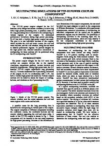
1.2.2 Secondary emission yield The ratio of secondary electrons to primary electrons is called the Secondary Emission Yield (SEY or Æ ). It is a property of the surface-material. Furthermore it depends on the kinetic energy and on the angle of incidence of the primary electron. Figure 1.1 (taken from [3]) illustrates the in uence of the kinetic energy of the primary electron. It shows the SEY for perpendicular incidence on an untreated copper surface. Apparently, if the primary electron is too slow (energy smaller than about 30 eV), the SEY is very small and does not even exceed unity. The same applies if its energy is too high (usually above a few thousand eV). 4
2.5 2.3
SECONDARY ELECTRON YIELD
2.1 1.9 1.7 1.5 1.3 1.1 0.9 0.7 0.5 0
500
1000
1500
2000
2500
3000
Energy (eV) Figure 1.1
Secondary emission yield of copper (from [3]).
Increasing angles of incidence #i of the primary electron (with #i = 0 being perpendicular to the surface) tend to shift the SEY curve towards higher yields. Several formulas have been proposed to describe this characteristic [35],[8],[50],[45],[6]. They mostly assume a SEY proportional to 1= cos(#i ), but are limited to cos(#i) < 0:2 to avoid unphysically high yields. 4
It is also known as Secondary Electron Yield, or simply Secondary Yield.
13
However, since the exact SEY is material dependent it is strongly a�ected by the properties of the surface. The latter can rarely be determined with certainty, because it changes during the operation of the device (e.g. due to outgassing, surface scrubbing by impinging electrons), and therefore the exact prediction of the SEY is very diÆcult. 1.2.3 Energy and direction of emitted electrons
When secondary electrons leave the surface they have an initial velocity of ~v . The velocity-magnitude v { usually expressed as initial energy W { is not the same for all electrons, but distributed as shown in Figure 1.2 (taken from [19]). Neglecting the backscattered electrons, the position of the maximum depends very little on the energy of the primary electron. Typically, the spectral energy distribution is peaked around 2 eV and the average energy is 4-5 eV [35]. 0
0
0
Initial energy of secondary electrons for primary electrons impinging with 175 eV (from [19]). The peak at 175 eV (W ) represents re ected electrons. Figure 1.2
f
The direction of the emitted secondary electrons is expressed by the angle with respect to the surface normal. It follows a cos(#e) distribution, hence the direction normal to the surface is prefered [50]. Some multipacting computer codes employ this distribution [48],[12], others make the simpler approach of emission perpendicular to the surface [24]. #e
14
1.3 Multipacting 1.3.1 Development of an avanlanche Electrons from beam loss, residual gas ionization and other processes can produce free electrons in a RF cavity. Driven by the electromagnetic forces these electrons will sooner or later hit the boundary. Due to the impact secondary electrons might be released. They are again driven by the electromagnetic forces and will also hit the cavity wall, producing even more secondary electrons. Certain con gurations allow the electron trajectories to be recurrent. These trajectories form so called closed paths. The number of participating electrons is then increasing exponentially. For such a multipacting discharge to be self-sustaining a number of conditions have to be ful lled [10]. 1.3.2 Conditions Kinematic criterion
To assure that the electron trajectories combine to a closed path, the impact point of one partial trajectory must coincide with the launch point of a preceding trajectory. This coincidence must be both in place and in the phase of the RF eld. The coincidence of the phase requires that an integer number of RF cylces elapses between launch and impact. The number of RF cycles is called the order of multipacting. Another technical term refers to the number of impact places hit during one orbit of the closed path. If the electron returns immediately to its origin, the process is called single surface multipacting or one point multipacting. In case there are two di�erent impact places involved (e.g. the discharge between parallel plates) the process is called two point multipacting. This denomination can of course be extended to n points. Unfortunately, there also exist closed paths consisting of two or more partial trajectories that concern a single surface only. The electrons impact a single place several times at di�erent RF phases until they meet the original phase again. The denomination as one point multipacting of n order is confusing since a single electron which returns to its initial site (place and phase) after n RF cycles would be given the identical name. In [38] an approximate division of the order of multipacting into the corresponding orders of the partial tracks (e.g. 2 + 2=3 + 1=3) has been proposed. The complexity of a closed path is then directly connected to the lenght of its name. In a subsequent chapter an example will be given. th
15
Stability criterion
It has been mentioned in section 1.2.3 that the initial energy of the secondary electrons is not a xed value. This fact results in slight variations of the time of ight [10]. Therefore it is not an in nitesimal thin sheet but a more or less compact cloud of electrons which follows the path prescribed by the kinematic condition. Moreover, space-charge forces tend to disperse this electron cloud. For the electron avalanche to hold over a considerable number of cycles an inherent phase focusing or self-adjustment of the transit time is necessary, so that nearly synchronous electrons are pulled in towards the synchronous condition [44]. The range of RF phases around the synchronous phase which are subject to such a focusing process is called the capturing range. It does not only sustain a resonant discharge, but it also increases the chance that free electrons can trigger it. 5
Criterion for electrons to escape from the surface
As mentioned before a closed path can consist of several partial trajectories. For this to be possible all the secondary electrons knocked out by an intermediate impact must be able to lift o� from the surface. Usually it is a condition to the electric eld to point into the right direction. But secondary electrons can also be ejected into an opposing eld if their initial energy is suÆciently high [16]. This happens, for instance, in regions of low electric eld or shortly before the zero crossing of the electric eld (e.g. � = !t = 0; �; : : :). Physical criterion
A fundamental property of a multipacting discharge is the exponential increase of the number of participating electrons. Therefore the total amount of secondary electrons generated during one orbit of the closed path must exceed unity; hence the product of the secondary emission yields for all impacts during one orbit must be greater than one. 1.3.3 Notes on multipacting in RF cavities It is sensible to divide the conditions introduced in the previous section into two categories. While the rst 3 conditions concern the elds and thus the geometry of the resonant cavity, the last (the physical condition) is a condition of the surface material. When suppressing a multipacting discharge, a geometrical solution is in general preferable to any surface treatment [44]. Thus, \Synchronous" means: in synchronism with the electromagnetic eld, to ful ll the kinematic condition. 5
16
the rst category of conditions is considered the most important because of its independence of the material. When an electron is launched from the surface, the shape of its trajectory is dictated by the local eld. Therefore each point on the surface has its own characteristic with respect to the kinematics of electrons. A global in uence exists only due to the eld's amplitude (the power applied to the device). It is known from practical experience that multipacting discharges occur in bands with respect to the amplitude of the eld. Certain bands can promote multipacting, others not. Numerical investigations have shown that each band can be traced back to a discharge at a certain position on the surface and of a certain type and order. The most frequent type is one-point multipacting. Its trajectories do not penetrate very deep into the cavity. It is obvious that they mostly depend on the local eld con guration [43], [42]. For a given position showing a speci c type of discharge (e.g. one point multipacting) the process of rst order is always the one with the highest eld amplitude. A discharge of the same type but higher order appears at a lower eld level; hence it forms another band. Theoretically there does not exist a lower limit for the eld, because the order can be increased until in nity. 6
1.4 Example { multipacting between parallel plates To illustrate all of the above-mentioned terms a simple example is presented here. It is the two-point multipacting between parallel plates. In [23] it has been calculated for the rst time. Solution of the equation of motion Consider two parallel plates at x = 0 and x = d (Figure 1.3). Applying an alternating voltage with amplitude U produces a homogeneous electric eld 0
~ (t) = U0 E d
sin(!t)(
~ 0 sin(!t); ~ex ) = E
where ~ex is the unit vector along the x-axis. For the analytically solved two-point multipacting between parallel plates it is easy to check that higher order multipacting processes can at least ful ll the kinematic condition. For other geometries this is not proved. 6
17
x=d
E0sin(wt)
x=0 Figure 1.3
Multipacting between parallel plates.
The electric eld forces the electrons to bounce back and forth between the plates. There is no magnetic eld, simplifying the solution of Equation (1.1). Integrating it two times yields the position x(t) of the electron x(t) =
eU0 � ! (t t0 ) cos !t0 +sin !t0 me ! 2 d
�
sin !t +(t
t0 )x_ (t0 )+ x(t0 ):
(1.3)
Denoting the phase of the RF eld at the launch of an electron as !t = � , setting the starting location to x(t ) = 0, and setting the initial velocity of the electron x_ (t ) = 0 (to simplify matters) one gets 0
0
0
0
x(t) =
eU0 � (!t me ! 2 d
�0 ) cos �0 + sin �0
�
sin !t
(1.4)
:
Now the conditions given in section 1.3.2 will be applied. Kinematic condition To ful ll the kinematic condition the ight time of an electron (!t � ) until it returns to x = 0 must be equal to 2n�, with the parameter n denoting the order of multipacting. Thus n counts the number of RF cycles elapsing until the electron returns to the point where it was launched. Before its return to x = 0 the electron hits the plate at x = d. The process is therefore called two-point multipacting. Since the eld is homogeneous, both electrodes are interchangeable. As a consequence, it is suÆcient to deal with the rst partial trajectory only, i.e. the ight from x = 0 to x = d. The kinematic condition then requires that the electrons reach the opposite electrode after an odd number of half-cycles. It reads !t � = (2n 1)�: (1.5) 0
0
18
Putting this into Equation (1.4) and rewriting sin(� + � ) as sin(� ) yields 0
d=
eU0 � (2n me ! 2d
1)� cos � + 2 sin � 0
�
0
0
:
One can now derive a relation between the Voltage level U and the initial phase � that ful lls the kinematic condition: me (!d) U = : (1.6) e (2n 1)� cos � + 2 sin � 0
0
2
0
0
0
Escape from the surface For the electrons to escape from the surface at x = 0 the initial phase must be restricted to 0 � � < 180 degrees. The escape of the electrons from the upper plate is then guaranteed by the ight time being an odd number of half-cycles. When the electron hits the electrode at x = d the electric eld has reversed, so that the electron meets the same conditions as in x = 0. 0
Stability The evaluation of the stability of the electron trajectories is more complicated. According to [23] the curve given by Equation (1.6) consists of two branches. For initial phases � smaller than a critical phase �c it is attractive; that is electrons starting nearby the resonance are pulled in towards the resonance. For initial phases � > �c the curve becomes repelling, and only those electrons strictly satisfying Equation (1.6) stay at their initial phase. Electrons starting with phases beyond the unstable branch drift further away and nally stick to the surface. At initial phases smaller than the repelling branch electrons get captured by the stable branch. The critical phase �c is characterized by the coincidence of the stable and the unstable branch and by a minimum of U . For the rst order (n = 1) multipacting band �c is 32.5 degrees. At � = 0 the stable branch vanishes, and Equation (1.6) gives an upper limit for U . These results have been applied to an electrode separation of 28 cm and a frequency of 88 MHz. They are illustrated in Figure 1.4. The gray shade represents the capturing range. It should be noted that [23] also mentions the possibility of electrons being captured though their initial phase was beyond the unstable branch. Those additional capturing regions are not closed by attractive or repelling phases. The captured electrons nally end up on the stable branch between 0 and �c. Unfortunately, no further quantitative information has been given. 0
0
0
0
0
19
50 48 46 upper limit
U0 [kV]
44 42
← stable (attractive) unstable (repelling) →
40 38
φc
36
lower limit
34 32 0
10
20
30
40
50
60
70
80
90
Initial phase [deg]
First order multipacting between parallel plates, kinematic condition and stability for f=88 MHz and d=0.28 m. Figure 1.4
Physical condition To apply the physical condition, the arrival velocity of an electron has to be calculated. Knowing the SEY of the electrodes one can then narrow the range of eld levels (and initial phases) for which multipacting is possible. To obtain the velocity of an electron upon arrival at the opposite plate Equation (1.4) has to be derived with respect to the time. Then the kinematic condition for the ight time ( Equation (1.5) ) is to be employed again. Rewriting cos(2n� � + � ) as cos � gives the velocity at impact e x_ (t = timp ) = vimp = 2 U cos � : (1.7) me !d The impact energy Wimp of the non-relativistic electron then reads as follows (in eV): e Wimp = 2 U cos � : (1.8) me (!d) Using the numbers from Figure 1.4 it can easily be veri ed that the energy of the electrons is too high to produce a suÆcient number of secondary electrons. Table 1.1 lists a number of values for some combinations of resonant initial phase and corresponding voltage. No multipacting is possible because the physical condition is not ful lled. 0
0
0
2
20
2 0
2
0
0
Impact energies of resonant electrons (theory). � U Wimp [deg] [kV ] [eV ] 0 43.38 27615.5 10 39.6 22322.5 32.5 36.59 13978.0 55 39.61 7576.2 65 43.4 4936.3 Table 1.1
0
0
21
Chapter 2 Numerical treatment of multipacting 2.1 Overview { tasks of a computer code The solution of the equation of motion (1.1) becomes rapidly complicated if magnetic elds are involved or if the elds are inhomogeneous. To attempt an analytical solution for an accelerating cavity is hopeless, if not impossible. At this point it becomes inevitable to make use of the opportunities a computer o�ers. Apart from calculating the elds in a given geometry it is used for the following two tasks: 1. Solution of the equation of motion by integrating it with respect to time. During the integration { which is basically tracking the electron for each timestep { the trajectory is monitored for hitting a boundary. Secondary electrons are generated and tracked if necessary. 2. Analysis of the calculated trajectories to give the user a hint where to expect multipacting. Resonant trajectories are de ned by a set of 3 parameters (x , E , � ) which have to be determined. 0
0
0
While the rst point can easily be handled with standard integration algorithms (e.g. Runge-Kutta), for the latter some new means have been developed by Somersalo et.al. [38], [40]. It should be emphasized in advance that the results of a computer code can only serve as a hint. They have to be interpreted carefully. 22
2.2 Solution of the di�erential equation 2.2.1 Underlying ideas Ordinary higher order di�erential equations can always be reduced to a set of coupled rst-order di�erential equations. Numerial methods usually solve this set of coupled equations. The equation of motion, which is of second order, is therefore reduced to a set of two rst-order di�erential equations. For non-relativistic electrons it reads as follows: � � d~v(t) e E ~ (~x; t) + ~v (t) � B ~ (~x; t) = me dt (2.1) d~x(t) = ~v(t): dt The usual way of specifying the boundaries is to give the position ~x and the velocity ~v of an electron for some starting point t = t . This makes the di�erential equation an initial value problem, which can be solved by integration with respect to time. The result is called the trajectory of the electron. The calculation has to be abandoned if the electron attempts to \cross" the boundary, i.e. if it impacts the surface. The position of the impact can then serve as initial position for the trajectory of a secondary electron. Two algorithms that perform the integration will be presented in the following sections. The underlying idea of any of these routines is to rewrite dv , dx and dt as nite steps �v , �x and �t, and then multiply the equations by �t. This gives algebraic formulas for the change in velocity and position when the time t is increased by one stepsize �t [36]. 1
0
2.2.2 Euler's method and general single step methods The so called Euler method is the literal implementation of the procedure described before. It results in Formula (2.2). ~v(t + �t)
= ~v(t)
�
�
e ~ ~ me E (~x; t) + ~v(t) � B (~x; t)
~x(t + �t)
� �t
(2.2)
= ~x(t) + ~v(t) � �t: This formula is unsymmetrical. The solution is advanced through an interval �t, but only the derivative information (the right hand side of the
Actually, it is a set of 6 equations since each component of the vectors yields a single equation. 1
23
equation of motion) at the beginning of the interval is used. It is obvious that only a small stepsize can provide a passable approximation [32]. Generally speaking, Euler's method is not the rst choice for the general purpose because it is neither very accurate nor very stable compared to other methods [36]. However, multipacting is a physical process with an inherent stability; that is resonant trajectories are insensitive to variations of the initial conditions. When analysing multipacting one is not interested in unstable non-resonant trajectories but in the identi cation of resonant trajectories. Therefore even a coarse method such as Euler's method is expected to give reasonable results, provided the stepsize is chosen suÆciently small. Euler's method is a single step algorithm, i.e. information about the derivative is needed only once per time-step. The general form of such a single step algorithm is y (x + h) = y (x) + h � �(x; y (x); h; f );
(2.3)
where x is the independent variable (e.g. the time t), h is the stepsize and f = f [x; y (x)] is the right hand side of the di�erential equation. Euler's method thus uses [32] �(x; y(x); h; f ) = f [x; y(x)]:
(2.4)
The evaluation of the right hand side of the equation of motion requires an interpolation of the electric and magnetic elds. The (perhaps only) advantage of single step algorithms is that these interpolations have to be done only once at each time step, which makes them faster than other methods. 2.2.3 Runge-Kutta methods and adaptive stepsize control To overcome the unsymmetry of Euler's formula ( Equation (2.2) ) and thus improve the numerical solution, Runge-Kutta methods take several Euler style trial steps over the interval, and then combine the information obtained to match a Taylor expansion up to a certain higher order. The Runge-Kutta algorithms are distinguished according to the order of the truncation error. A method is conventionally called n order if the error term is O(hn ) [36]. The classical fourth-order Runge-Kutta, for instance, evaluates the right hand side of the di�erential equation four times: once at the initial point, two times at a trial midpoint, and another time at a trial endpoint of the interval. The combination of these steps in the following manner yields an th
24
+1
error term O(h ): 5
k1 k2 k3 k4
= = = =
hf [x; y (x)] k hf [x + h 2h ; y(x) + k21 ] hf [x + ; y (x) + 2 ]
2
2
(2.5)
hf [x + h; y (x) + k3 ]
y (x + h)
= y(x) + k6 + k3 + k3 + k6 + O(h ): Runge-Kutta methods of order m higher than four require more than m evaluations of the right hand side f (though not more than m + 2) [36]. A fth-order method, for example, requires at least six evaluations of f . It therefore has some overhead as compared to the fourth-order method (2.5), and the latter seems to be preferable. But combining these six evaluations of f in a di�erent way, another fourth-order method can be derived. This fourth-order method is called embedded (in the fth-order method). The idea of such an embedded Runge-Kutta method is to monitor the accuracy of the solution by comparing the two methods, and then adapt the stepsize automatically in order to achieve a certain accuracy. Huge steps can be taken if the solution is practically linear, while many small steps should tiptoe through treacherous terrain [36]. The general form of a fth-order Runge-Kutta formula is k = hf [x; y (x)] k = hf [x + a h; y (x) + b k ] ... (2.6) k = hf [x + a h; y (x) + b k + � � � + b k ] y (x + h) = y (x) + c k + c k + � � � + c k + O(h ): The embedded fourth-order formula is y �(x + h) = y (x) + c� k + c� k + � � � + c� k + O(h ): (2.7) There exist several sets of parameters a, b, c and c� for fth-order RungeKutta methods and embedded fourth-order formulas [32]. Those found by Cash and Karp have been used subsequently (section 2.5). They are quoted in [36]. The advantage of Runge-Kutta methods is their robustness. It does not require very much knowledge of the stability of the di�erential equation to obtain good results. The high number of time consuming evaluations of the right hand side of the di�erential equation is compensated to a large extent by the automatically adapted stepsize, which saves a lot of calculation steps. 1
2
3
5
4
1 2
2
21
1
6
6
61
1
1
1
1
2
2
2
25
2
2
65
6
6
5
6
6
6
5
2.3 Means for predicting multipacting 2.3.1 Motivation and general idea The mere solution of the equation of motion is not very helpful to analyse a device for multipacting discharges. There are too many combinations of initial parameters which have to be tested. To be precise, it is rstly the initial velocity (or energy) and its direction, furthermore the initial position and the starting time (corresponding to an initial phase � of the RF eld), and nally { rather a global than an initial parameter { the amplitude of the RF eld. Even if the secondary emission properties are restricted to a xed initial energy (e.g. 2 eV) and a single direction of emission (e.g. perpendicular to the surface), there remain 3 parameters: x , � and E . To search for multipacting trajectories by manually varying these three parameters would be like searching the needle in the hay; perhaps even worse because it's not clear that it exists. For that reason it is necessary to provide some means to automate the search, that is some functions that result in a handy quantity used to decide whether a set of parameters is possibly resonant or not. All the existing means have to rely on the inherent self-adjustment of the transit time of a multipacting process. Electrons that start within the capturing range of a resonant discharge will be drifting towards the resonance. Outside the capturing range the electrons will show a number of irregular impacts, until they will nally stick to the surface because of the electric eld pointing into the \wrong" direction. 0
2
0
0
0
2.3.2 The electron counter The electron counter cn has originally been introduced by Somersalo et.al. [38]. Their approach was an application of ideas arising from the theory of dynamic systems. The principle of the electron counter is to single out the non-resonant trajectories on the basis of their nite number of impacts. The procedure works as follows: a huge number of electrons (e.g. 300000) is launched with two out of the three parameters chosen randomly or on a regular grid, while the third parameter is xed. The electrons are tracked, and for each impact a secondary electron is started. The calculation of an electron's path is stopped if it either sticks to the surface or if it reached a given number of impacts (n). Eventually, the number of electrons which survived n impacts is counted (cn). The secondary emission yield has been excluded here. In the limit of dealing with a very small number of electrons, the SEY has a negligible in uence on their trajectory. 2
26
This computation is repeated for di�erent values of the xed parameter. Usually it is the eld amplitude E which is stepped through an interval. The electron counter then is a function of the amplitude: cn(E ). It will have maxima and minima which correspond to high and low electron activity respectively. The maxima indicate the amplitudes of the eld that might be susceptible to multipacting. An example is given in Figure 3.13. 0
0
2.3.3 Spatial focussing { observing the particle distribution Spatial focussing is a somewhat misleading term. It originates from the fact that the kinematic condition requires recurrence of the initial parameters at re-emission. Unlike the phase of subsequent impacts, which is pulled in towards the resonance if it has initially been within the capturing range, the position of the impacts often drifts away from the resonance. That means that the position of a multipacting discharge is usually (weakly) repelling, whereas the phase is focussing. Nevertheless, the closer the initial position is to the resonance, the closer the impacts will be to the starting location. This can be observed in di�erent ways. The straightforward method is to calculate the distance between an impact and the initial position of an electron. A more visual approach is to track many electrons (e.g. 10000) with random initial position and phase in parallel, and then print their position to the screen. After a few RF cycles the region close to the resonance will still be teeming with electrons, whereas in other regions the electrons will have sticked to the surface (see Figure 3.14, for example). This procedure requires the amplitude of the eld to be xed to a value that is prone to multipacting. Otherwise nothing but \noise" will be observed. This functionality could in principle be included in the electron counter, if it stored all the trajectories (or at least their impacts) that survive n impacts. At a maximum of the electron counter an investigation of the trajectories should permit to locate the resonant position. 2.3.4 Phase focussing { visualization of the capturing range The direct method to pro t from the phase focussing of a multipacting discharge is to evaluate the di�erence between the RF phase at launch and subsequent (n ) impact of an electron's path. If the electron is started within the capturing range, and if it (and its succeeding secondary electrons) is given th
27
enough time to drift to the resonance, then the phase of the n impact will be equal to the resonant phase. The closer the launch is to the resonance, the smaller will be the di�erence between initial phase and impact phase. Outside the capturing range the impact phases are irregular, and therefore the di�erence to the corresponding initial phases is not a smooth function of the initial values. The electron might even be stuck to the surface by the electric eld before the n impact. A visualization of the capturing range requires the initial phase � to be stepped through an interval, while the other two parameters are xed. The di�erence between initial phase and impact phase is then drawn as a \function" of the initial phase. In spite of such a two-dimensional plot it is possible to create a grey or colour scale plot which allows to vary another parameter, e.g. the eld amplitude E . Figure 3.9b shows an example. th
3
th
0
0
2.3.5 The distance function The distance function dn is the combination of the means based on spatial focussing and phase focussing into a single quantity. Like the electron counter it originates from a team at Helsinki (Somersalo et.al. [38]). The idea is to compute an electron's path up to a given number of impacts n. At the n impact both the distance to the initial position and the di�erence between initial phase and impact phase are calculated. Both are combined to the distance function dn in the following manner: th
dn (~x0 ; �0 ) =
p
ei� j ; (2.8) where ~xn, �n denote position and phase of the n impact respectively, and � is a parameter used to adjust the weight of the phase di�erence and to adapt this di�erence to the unit meter. Obviously, the distance function is zero only if launch and impact of the electron's path coincide. Hence the distance function checks if the kinematic condition is ful lled. The smaller dn is, the closer the initial parameters are to the resonance. Usually two out of the three initial parameters are varied, while the third parameter is xed. For each set of parameters the distance function is calculated, and then a colour scale or grey scale plot is drawn. When using � and E as variable parameters a multipacting discharge is to be recognized by its capturing range on the �-scale and a certain bandwidth on the E -scale. Figure 3.9a shows an appropriate example. j~x
0
~xn j2 + � 2 jei�0
n 2
th
0
0
The di�erence of two phases is to be understood as �imp �� 2 [0; 360) and k 2 N0 . 3
28
�0
= �� + 2k�, where
2.4 Existing codes The rst numerical analysis of multipacting in a RF accelerating cavity has been carried out at Stanford University in the 1970's [31]. Since then a number of multipacting computer codes has been developed. The majority of these codes has been programmed for a single study only, and in some cases they have been adapted to di�erent geometries. In [28] an overview of existing codes is given. Only a very few of these computer codes are equipped with an interface to the general user, amongst them are MultiPac [48] and MultP [25],[24]. Both codes require a closer inspection; MultiPac because it has been developed by the inventors of the electron counter and the distance function and because of its Matlab interface, and the code MultP because of its capability to calculate electron trajectories in 3 dimensions. For the present work it was desired to analyse an axissymmetric RF cavity. The cavity was planned to be surrounded by solenoids creating a static magnetic eld along the cavity axis (z-axis). A future analysis should also include this solenoidal eld, thereby imposing the necessity of 3D calculations. The reason can easily be seen from the components of the electromagnetic forces given in cylindrical coordinates in Equation (2.9). The components introduced by the static magnetic eld are bold-faced. F% / E% + ( ' z vz B' ) v% z (2.9) ' / Fz / Ez + v% B' : The magnetic eld of an axissymmetric RF structure has a '-component only, while the electric eld has a %- and a z- component. Assuming that the initial velocity of the electron is perpendicular to the surface, hence it has no '-component, the force is restricted to be within the %-z plane. An ordinary axissymmetric structure can therefore be treated as a 2D problem. The magnetic eld of the solenoids, however, introduces a Bz -component. This entails a '-component of the force which kicks the electron out of the %-z plane and adds a '-component to the velocity. A calculation in all three dimensions is thus necessary. It is for this reason that the MultP code has been given preference. It was available at CERN, and a contact to the programmer Sergej Tarassov has been established. The MultiPac code, on the other hand, was only available when this work was almost nished. It could therefore not be thoroughly 4
5
v B
F
B
Code developed at Rolf Nevanlinna Institute, University of Helsinki in collaboration with DESY, Hamburg. 5 Code developed at the Institute for Nuclear Research, Moscow. 4
29
tested. Fortunately, the authors of the code had well documented and published a number of sample calculations which served as a comparison.
2.5 Test code for two simple geometries 2.5.1 Motivation
Precompiled codes usually su�er from a lack of transparency. The user hardly ever knows what the code is really doing. He can only compare the output to theoretical predictions or to the results of proven codes. If the results do not stand the comparison, in many cases one can only guess the origin of the failure. To overcome this problem, and to gain a deeper understanding of the possibilities and limits of numerical simulations of multipacting a simple test code has been written in FORTRAN. It has been programmed for two geometries { the parallel plates and a coaxial resonator { whose elds are known analytically. 2.5.2 Characteristics of the test code
For the solution of the di�erential equation a fth-order Runge-Kutta method with embedded fourth-order formula based on Cash-Karp parameters was taken from literature [36]. It was assumed that this published algorithm had proven its reliability, so almost no modi cations were made to it, except for the implementation of a break-o� condition. This was necessary in order to stop the integration at an impact of the electron. A secondary electron then has to be generated at the impact position, and a new integration has to be started. The secondary emission yield was thus xed at unity. Beyond the mere integration the test code was programmed to output the electron's path, to calculate the impact energies and to compute the distance function. For a single electron path the initial energy W , position x , phase � and the eld amplitude E are adjustable. The distance function is based on these trajectory calculations, with initial phase and eld amplitude being varied in adjustable intervals. A number of preliminary simulations revealed that the parameter � of the distance function in uences the contrast of the plot only, so it was eventually set to 0.1. 0
0
0
30
0
2.5.3 Implementation issues The implementation of the break-o� condition requires two items to be thought out: the calculation of the impact point and the launch of secondary electrons. Both are covered in this section. Calculation of the impact point
The rst item is the exact calculation of the impact position, that is to say the formulation of the stopping condition. It is clear that the integration has to be stopped if an electron leaves the geometry. The exact position of the impact then has to be found between the position of the last and its preceding step. Many codes connect these two points with a straight line, and then de ne the position of the impact as the point of intersection of the straight line with the (parametrized) curve of the surface. By this method no further integration steps need to be taken, and thus time is saved. For the test code, however, a di�erent approach has been chosen to get a more precise value for the impact position. In fact, it is a bisection algorithm. The last step of the integration (which runs out of the geometry) is rejected, and the step is taken again with half of the stepsize. If the new point is inside, another step has to be taken with the same stepsize. If it ends up outside, the point is rejected and the stepsize halved again. This procedure is repeated until the distance between the positions of two successive steps is smaller than 10 m, but at most 20 trial steps are taken. The algorithm avoids the parametrization of the surface (which might be diÆcult if the code had to be adapted to a geometry that is more complicated than the parallel plates or the coaxial resonator). On the other hand, the number of RungeKutta steps to be taken is increased by it. But since the elds are given analytically, some 10 or 20 additional steps do not increase the computation time signi cantly. 7
Launch of secondary electrons
The next item concerns the condition for the secondary electrons to escape from the surface. The decision of whether or not to launch a secondary electron has to be formulated as a quantitative expression, so that the test code can evaluate it. In case of zero initial energy it is as easy as determining the direction of the electric eld. Electrons can only lift o�, if the electric eld points towards the surface. The code MultiPac even uses this simple critereon for non-zero initial energies. But with an initial energy of a few eV electrons can also be ejected into an opposing eld. Therefore a di�erent criterion is needed. 31
One approach (used by MultP) is to start the electron in any case, and then wait for its impact. If the phase of the impact is very close to the initial phase (a di�erence of a few degrees only), then it is very likely that the electron can not escape and that its path has to be terminated. Unfortunately, in a few cases electrons are hovering above the surface for more than 10000 integration steps until they nally impact the surface. To avoid this enormous waste of computing time the test code has been equipped with a di�erent criterion, in addition to the simple check of the direction of the electric eld. It prevents the launch of slow electrons into a strongly opposing eld. The test code de nes a "restoring" velocity that the electron would have reached if the current electric eld were constantly applied for a certain time. This velocity is compared to the initial velocity of the electron. The electron is launched if its initial velocity is superior to the "restoring" velocity. Preliminary simulations have shown that the application of the current electric eld for 1/20 RF cycle results in a good launch restriction. Thus, in order to escape from the surface an electron with initial energy W needs to satisfy the condition r 2eW e 1 E~ � ~n � 0; (2.10) me me 20f where ~n is the vector normal to the surface. Clearly, this calculation is fairly arbitrary and does not reproduce the correct physical behaviour, but it avoids the unnecessary and time consuming integration, and it is closer to physics than a simple check of the eld direction. 0
0
2.5.4 Veri cation of the test code Even the most carefully programmed computer code can produce erroneous results. Therefore a number of numerical experiments were carried out to verify the test code. At rst a comparison with the analytical solution of the parallel plates was made. Secondly, the test code was compared to the results from the multipacting simulation of a coaxial cable (calculated with MultiPac). And nally some additional experiments were made to illustrate the e�ect of the non-relativistic approximation of the equation of motion and of certain simpli cations of the secondary emission process. Multipacting between parallel plates
The trajectory of an electron moving in a homogeneous electric eld is one of the simplest trajectories imaginable. In space it is represented by a straight 32
line in parallel with the electric eld lines. Errors in the numerical solution are more likely to a�ect the time dependence of the electron's position than the spacial shape of the trajectory. It is therefore reasonable to limit a veri cation of the numerical results to a comparison of phase and energy of the impacts with the analytical solution. Unfortunately, to select a number of representative initial parameters for comparison poses a major problem. Because of the trancendental nature of the trajectory equation ( Equation (1.4) ) [33] it appears to be an impractical goal to obtain a closed expression for the impact phases for any arbitrary initial phase and eld amplitude. Bearing in mind Figure 1.4 a di�erent approach was chosen. The impact phases shall not be compared directly, but the resonant { or non-resonant { behaviour of the electrons shall be compared to theory. In order to visualize the capturing range of a multipacting band, the distance function is calculated. The number of impacts is set to 30, so that the electrons can all drift to the resonant phase. Frequency and distance of the plane parallel plates are chosen according to the analytical example (d = 28 cm and f = 88 MHz), as well as the initial velocity (v = 0). Figure 2.1 shows the rst-order multipacting band calculated with the test code. The graph is black where the distance function is at its minimum (=0). The lighter the shade is, the bigger is the distance. White areas correspond to electron paths that did not survive 30 impacts. The solid line represents the exact resonant phase obtained from Equation (1.6). Apparently, the numerical calculation is in very good agreement with the theoretical prediction. The only di�erence are the grey stripes beyond the unstable end of the capturing range. They are caused by trajectories which start with a few irregular impacts, but nally get into the capturing range. This behaviour had already been predicted (but not quanti ed) in [23]. Beside the resonant behaviour also the energy of the impacting electrons is of big interest, because it in uences the number of secondary electrons that can be produced. Table 2.1 lists some impact energies of resonant trajectories. The initial parameters have been chosen from the solid line in Figure 2.1 (given by Equation (1.6) ); theoretical predictions for the impact energies have been obtained from Formula (1.8). A brief comment on Table 2.1 has to be made concerning the initial phases 55 and 65 degrees. These values are situated on the unstable branch of the resonance, hence the succeeding impacts drift away from the initial phase. Even though the numerical calculation has been abandoned after the rst impact, an exact coincidence of initial phase and impact phase could not be achieved. As a consequence also the impact energies must di�er. The result is nevertheless very encouraging. 0
33
50 48 46
U0 [kV]
44 42 40 38 36 34 32
0
20
40
60
φ [deg.]
80
100
120
0
Distance function for the 30th impact for parallel plates (d=28 cm, f =88 MHz), calculated with the test code and compared to theory (solid line). Above 120 degrees no electron survives 30 impacts. Figure 2.1
Impact energies of resonant electrons between parallel plates (theory versus test code). � U Wimp (theory) Wimp (test code) [deg] [kV ] [eV ] [eV ] 0 43.38 27615.5 27615.5 10 39.60 22322.5 22322.5 32.5 36.59 13978.0 13977.9 55 39.61 7576.2 7576.06 65 43.40 4936.3 4936.35 Table 2.1
0
0
34
Multipacting in coaxial resonator
A second check for the multipacting test code is the comparison with the results of the MultiPac code. Actually, the initially inconsistent outputs from MultP necessitated these additional calculations. Thanks to these calculations the origin of MultP's faulty results could be found. Unfortunately, an attempt to get hands on the code MultiPac was only successful half a year after these investigations were carried out. So the present work had to rely on the results published in [38],[39],[47] and [40]. Luckily, they were very well documented. The authors had investigated multipacting in a coaxial resonator whose electromagnetic elds can be described analytically. To compute electron trajectories with the test code, analytical elds were a substantial prerequisite since the test code did not include an interpolation algorithm to import eldmaps from an external eld solver. The coaxial resonator was designed for a resonant frequency of 1.3 GHz. The radius of the inner conductor was a = 8:7 mm, the outer shell had a radius of b = 20 mm. The length of the resonator was l = 2� = 461:2 mm, but for symmetry reasons the analysis could be restricted to �=4 � z � �=2. The electromagnetic elds are given by U ~ (%; z; t) = E sin( !c z) sin(!t + � )~e% % � ln(b=a) (2.11) U ~ (%; z; t) = cos( !c z) cos(!t + � )~e'; B % � c � ln(b=a) where c is the velocity of light, ! = 2�f is the angular frequency and %, ' and z are the cylindrical coordinates. Since the MultiPac code scales the eld amplitude of its outputs in units of input power P , the test code had to be adapted. The voltage U between inner and outer shell is related to the average input power P as follows [38]: p U = 4 � 120 � P ln(b=a): (2.12) In addition to the scaling of the eld amplitude a few more properties of the test code had to be altered in order to compare it to MultiPac. The most substantial change was to integrate the relativistic equation of motion (Equation (1.2) ), instead of its non-relativistic approximation. Moreover, the condition to launch a secondary electron had to be restricted to a simple check of the direction of the electric eld. Though MultiPac launches electrons with an initial energy of 2 eV, it does not consider the possibility to launch electrons into an opposing eld. At rst a single resonant electron trajectory is compared (Figure 2.2). This trajectory is of the one point type, and according to [38] the order is 1+1. 0
0
0
0
0
0
0
0
0
35
Both trajectories { the rst calculated with MultiPac and the other obtained from the test code { are almost identical. There is only a small di�erence in the impact phases. MultiPac calculates the impacts up to 1.5 degrees \later" than the test code, and therefore ful lls the kinematic condition at a slightly higher phase. This is partly due to the di�erent integration algorithms (MultiPac uses a 3 to 4 -order Runge-Kutta scheme), and to the di�erent ways of calculating the exact impact point (linear interpolation versus bisection). 6
rd
th
0.02 0.019 0.018 Radial position [mm]
0.017 0.016 0.015 0.014 0.013 0.012 0.011 0.01 0.009 0
200
400
600
Phase [deg]
(a) Computed by MultiPac, impact phases 74 deg and 54 deg (from [38]).
(b) Calculated by test code, phases drift to 72:5 deg and 52:9 deg.
Resonant electron trajectory in a coaxial resonator (electron starts from the outer shell at z = �=4, � = 54 deg, P = 610 kW). Figure 2.2
0
0
0
As pointed out in [38] the only position to show resonant trajectories is at z = �=4 = 57:65 mm, where the magnetic eld vanishes. Starting from any other point z 6= �=4 the electrons tend to drift towards the end of the coaxial resonator where they nally die. Thus the magnetic eld in uences nonresonant trajectories only. An example of those, however, is not yet published in literature. Therefore the e�ect of the magnetic eld could only be veri ed Comparisons of other resonant trajectories partly yielded bigger di�erences, but no more than 5 degrees. 6
36
qualitatively by the observation of electrons being pushed out towards the end of the resonator. The test code has reproduced this behaviour very well; Figure 2.3 shows an appropriate example. 20.0 19.0
Radial position [mm]
18.0 17.0 16.0 15.0 14.0 13.0 12.0 11.0 10.0 9.0 62.0
63.0
64.0
65.0
66.0
67.0
68.0
69.0
70.0
z [mm]
Non-resonant trajectory drifting towards the right end of the coaxial resonator (z =�=4 + 5 mm, � =54 deg, P =610 kW). Figure 2.3
0
0
0
In order to evaluate the e�ect that di�erent impact phases (of MultiPac and the test code) can have on the recognition of multipacting discharges, the distance function has been calculated. To include one-point multipacting, such as the process illustrated in Figure 2.2, the initial position has to be set to the outer shell at z = �=4. Figure 2.4 shows the results of both codes. Two characteristics of the plots need further explanation: rstly, the plot of the test code has a darker shading. This is due to the di�erent preparation of the plots (with Matlab). The authors of MultiPac have simply brightened up their result a bit more and have given it a higher contrast. Secondly, the test code lacks some multipacting bands below 50 kW. This is caused by a restriction of the test code to multipacting of 8 order (for time constraints). Apart from that, the grey scale plots obviously coincide. Hence it is safe to conclude that the small di�erences in impact phases can be neglected. Incidentially, there is an interesting annotation to be made on the resonant trajectories shown in Figure 2.2. The fact that the electrons have an intermediate impact before they return to their initial phase is also re ected in the distance function. It can be seen in Figure 2.4 that the resonant phase of the highest multipacting band (600 to 700 kW) splits into two branches. th
37
120
100
phase [deg]
80
60
40
20
0
100
200
300
400 power [kW]
500
600
700
600
700
(a) Calculated by MultiPac [38]. 120
100
φ0 [deg.]
80
60
40
20
0 0
100
200
300
400
500
P0 [kW]
(b) Calculated by the test code. Figure 2.4
Distance function d in the coaxial resonator. 38 30
These minima of the distance function do not correspond to two seperate resonant trajectories but to a single path of the more complicated order 1+1 [38] [42]. The conclusion to be drawn from these comparisons is, that the test code is capable of correctly reproducing the multipacting processes both between the parallel plates and in the coaxial resonator. It shall therefore be used to carry out two additional experiments, and it shall be used in the next chapter to verify the results produced by MultP. 2.5.5 Additional numerical experiments As stated in [29] the initial energy of the electrons a�ects the probability to trigger an avalanche. The rst experiment will therefore be the launch of electrons into an opposing eld. Up to now only the direction of the electric eld was used to check whether or not an electron can escape from the surface. With the application of an enhanced launch condition ( Equation (2.10) ) this simpli cation is now revised. Again, the distance function is calculated for the 30 impact, and the initial energy is 2 eV. The result is presented in Figure 2.5. The most apparent e�ect is the widening of the multipacting th
120
100
80
40
0
φ [deg.]
60
20
0
−20
−40 0
100
200
300
400
500
600
700
P0 [kW]
Distance function d in the coaxial resonator, with secondary electrons being launched into an opposing eld.
Figure 2.5
30
39
bands around 350 kW and around 500 kW. Moreover, the capturing range of almost all bands is expanded, thus increasing the probability to trigger the resonant discharge. A second experiment aims to evaluate the e�ect of the non-relativistic approximation. Figure 2.6 shows the distance function for the 30 impact after integration of the non-relativistic equation of motion. It has to be compared to Figure 2.5 which was based on the relativistic di�erential equation. There are no signi cant di�erences in these two graphs, but only a slight shift of the multipacting bands towards lower eld intensities. th
120
100
80
φ0 [deg.]
60
40
20
0
−20
−40 0
100
200
300
400
500
600
700
P0 [kW]
Distance function d in the coaxial resonator, using the non-relativistic equation of motion.
Figure 2.6
30
40
Chapter 3 The computer code MultP 3.1 Overview The computer code MultP is a tool to support the analysis of multipacting in fully 3 dimensional resonant RF structures. Its development dates back to the early 1990's, when it has been applied to the multipacting analysis of a proton accelerating cavity at DESY [17]. Since then it has been modi ed for various other studies, and several publications have followed ([26],[25],[24],[27] etc.). MultP does not compute the electromagnetic elds of the device to be analysed. An external solver is needed for this task, whose eldmap is imported and interpolated. MultP then solves the non-relativistic equation of motion. In addition, it contains some functions to analyse the electron trajectories in order to search for multipacting. Nevertheless, the version available at CERN was not fully functional, and contained several bugs which had to be xed. The following chapter covers the checkup of MultP's di�erent stages of multipacting analysis and the modi cations that have been applied to the code.
3.2 Representation of the geometry The following example explains how MultP represents the geometry of the simulation volume. MultP uses 3 sectional planes onto which both the geometry and the electron trajectories are projected. Any object before a plane (i.e. x > 0, y > 0 and z > 0) is projected onto this plane. As a consequence, electrons seem to move within a metallic obstacle, such as the inner conductor of the coaxial resonator, though they are in fact moving before it. Figure 3.1 illustrates this procedure, and Figure 3.2 shows the output of MultP. The green areas represent metallic parts of the geometry that are 41
surrounded by vacuum (here the inner conductor), whereas black areas are completely outside the geometry. The red line and the blue dot represent an electron trajectory. 1
Projection of an electron in a coaxial resonator to three sectional planes. Figure 3.1
3.3 Import of eldmaps The transfer of eldmaps from the external solver to MultP is done with the aid of text les. MultP reads the eld quantities from an ASCII-encoded le, and then it interpolates the values onto its own grid. These grid cells are of cubical shape, and their dimensions can be adjusted. When MultP solves the equation of motion it must interpolate the elds again. This time the elds are needed at every position where the right hand side of the di�erential equation is evaluated. The quality of these interpolations was subject of the following investigation. 3.3.1 MAFIA eldmaps It is obvious, that already the export from the external eld solver must be well-thought-out. The description of the MultP code [24] suggested to use MAFIA for the computation of the eldmap. The coaxial resonator has therefore been discretized and computed with MAFIA, and the eldmap has Note that all three views are speckled with small grey dots. Those small dots do not represent electrons! They are just noise and result from the way MultP creates these projections. 1
42
MultP's three sectional views of the coaxial resonator with electron trajectory. Figure 3.2
43
been exported to a text le. A second text le containing the homogeneous eldmap of the parallel plates has been created "by hand" (with the help of a little FORTRAN code). Both les have then been imported by MultP. A rst attempt to calculate electron trajectories yielded realistic results for the parallel plates, while the trajectories in the coaxial resonator (based on the MAFIA eldmap) were of markedly unphysical nature. According to theory the electrons should stay in the %-z plane. But as the trajectories shown in Figure 3.3 demonstrate, a ' component of the force made the electrons move around the inner conductor.
Unphysical electron trajectories when using MAFIA eldmaps. Figure 3.3
It did not require much e�orts to nd the source of these errors. MAFIA uses a rectangular mesh with diagonal llings. The curved surface of the rotational symmetric structure could therefore not be suÆciently well discretized (see Figure 3.4). In consequence, the electric eld had a '-component though it should have had a radial component only. Figure 3.5 shows the components of the surface- elds on the outer shell as interpolated by MultP. Electron trajectories are highly sensitive to eld errors, especially near the surface. Using a eldmap created by MAFIA the erroneous '-component can obviously reach the same order of magnitude as the radial component. The negative impact on the trajectories thus needs no further explanation. 3.3.2 SuperFish eldmaps In order to signi cantly reduce the eld errors near the surface, the mesh used to compute the electromagnetic elds had to be improved considerably. A proper discretization of the curved surface can only be achieved with
44
Electric eld in a coaxial resonator, computed by MAFIA. Figure 3.4
120 100
E [kV/m]
80 60 40 20 0 -20
Er
-40
Eϕ 0
10
20
30
40
50
60
Angular position ϕ [deg.]
70
80
90
Electric eld at the outer shell of the coaxial resonator as interpolated by MultP, based on MAFIA eldmap. Figure 3.5
45
meshpoints that coincide with the boundary, that is with a conformal mesh [9]. This, however, is something that MAFIA can not provide. Therefore a di�erent eld solver was chosen. A reliable computer code to calculate electromagnetic elds on a conformal mesh is SuperFish. It is restricted to 2 dimensions, hence dealing with rotational symmetric structures only. Both the coaxial resonator and the 88 MHz cavity (which was eventually to be analysed) are of this symmetry. Using SuperFish necessitates a transformation of the 2D output (of SuperFish) into a 3D eldmap for MultP. A small FORTRAN program was written for this task. It imports the 2D eldmap, turns it stepwise along the '-axis and transforms each component into the corresponding cartesian components. Figure 3.6 illustrates this procedure. Ex
Er Ey
Figure 3.6
Transformation from 2D Super sh eldmap to 3D eldmap.
The result has been a much better approximation of the elds near the surface. Figure 3.7 shows the improved eld-components as MultP has interpolated them from the SuperFish data. The '-component has been reduced by almost two orders of magnitude.
3.4 Trajectory calculation 3.4.1 Algorithm to solve the di�erential equation MultP integrates the non-relativistic equation of motion. It assumes the RF elds to be time harmonic, and it neglects interactions between the electrons
46
120
E [kV/m]
100 80
Er
60
Eϕ
40 20 0 -20 -40 0
10
20
30
40
50
60
70
80
90
Angular position ϕ [deg.]
Electric eld at the outer shell of the coaxial resonator as interpolated by MultP, based on SuperFish eldmap. Figure 3.7
themselves. The integration is performed by a single step algorithm. Its stepsize is initially adjustable and then constant throughout the integration. The default value is 1=720 of a RF-period, which corresponds to a phase angle of 0:5 deg. In contrast to the Euler method, MultP rst approximates the midpoint of an interval by assuming that the electron would y with constant velocity. Then it advances the solution over the interval �t, evaluating the right hand side of the equation of motion with the elds taken at the midpoint [41]. 3.4.2 Trajectories between Parallel plates
Like the veri cation of the test code the check of the trajectories calculated by MultP started with multipacting between parallel plates. Resonant phases and impact energies were compared with theoretical predictions. The initial phases and eld amplitudes were again calculated with Equation (1.6). MultP could exactly reproduce these resonances. The corresponding impact energies are listed in Table 3.1. They were very close to the theoretical predictions. The di�erences even dropped o� to the order 10 when the stepsize was reduced to 0:2 deg. But this e�ort did not pay, since it doubled the calculation time without increasing the accuracy signi cantly. 7
47
Impact energies of resonant electrons between parallel plates (theory versus MultP). � U Wimp (theory) Wimp (MultP) [deg] [kV ] [eV ] [eV ] 0 43.38 27615.5 27615.65 10 39.60 22322.5 22322.65 32.5 36.59 13978.0 13978.0 55 39.61 7576.2 7576.2 65 43.40 4936.3 4936.3 Table 3.1
0
0
3.4.3 Trajectories in the coaxial resonator Beyond the analytical example of the parallel plates also a few trajectories in the coaxial resonator were computed. Unfortunately, they cannot be compared to the results from MultiPac directly, because MultP xes the initial energy of the secondary electrons to zero while MultiPac launches them with 2 eV. Moreover, the trajectory plots of MultP do not show the electron's position, but only its distance from the initial position. Here the test code had to step into the breach. It has been adapted to produce an output similar to MultP. The eld amplitudes were converted according to Equation (2.12) from the power scaling that MultiPac had applied to scale the voltage between inner and outer conductor. Figure 3.8 compares a sample trajectory which has { apart from the initial energy { the same initial parameters as the trajectories shown previously in Figure 2.2. Both codes have produced an almost identical result. Though MultP seems to switch between two pairs of resonant phases, its impacts di�er by less than 5 degrees from the test code's values. These results indicate that MultP solves the di�erential equation correctly. 2
3.5 From phase focussing to the distance function 3.5.1 Phase- eld chart After having checked the solution of the di�erential equation the attention went to the analysis of the trajectories. MultP provides several functions to This applies to single electron trajectories only. In a subsequent section it will be shown, that MultP can calculate the distance function with initial energies greater than zero. But these trajectories can not be plotted as single electron trajectories. 2
48
|ρ-ρ0| [mm]
10.0 8.0 6.0 4.0 2.0 0.0 0
180
360
540
720
φ [deg.]
(a) Computed by the test code, phase drifts to 70:6 deg and 51:1 deg.
Resonant electron trajectory in the coaxial resonator, deg, P =610 kW ) U =15.612 kV.
Figure
�0 =54
(b) Computed by MultP, phase drifts to 66:5 deg =68:5 deg and 49 deg =54:4 deg.
3.8
0
0
facilitate the search for multipacting. Amongst these the so called \PhaseField Chart" is considered to be the most important. It makes use of the phase focussing process to visualize the capturing range of a resonant discharge. For this purpose MultP varies the initial phase and the eld amplitude within adjustable intervals, while the initial position of the electrons is xed. The di�erence between initial phase and impact phase is then presented in a colour scale plot. The minimum is coloured red, and with increasing di�erence the colour turns into blue. Provided the impacts of the electrons are very close to their initial position, the phase- eld chart is supposed to result in a diagram similar to the distance function { execpt for the little detail that colour is used instead of a grey scale, and that the axes are interchanged as against the preceding grey scale plots of the distance function. Test with the parallel plates
The rst test for the phase- eld chart were the parallel plates, as usual. It was expected that the result would be { to a certain extend { comparable with Figure 2.1, since the preceding section had shown that MultP reproduces the resonant trajectories correctly. It was therefore an enormous surprise to nd the phase- eld chart absolutely blank. Even the combinations of initial 49
phase and eld amplitude that are listed in Table 3.1 did not appear in the chart. Test with the coaxial resonator
From the blank phase- eld chart of the parallel plates it was hardly possible to draw any conclusion. Therefore another attempt was made with the coaxial resonator. To compare the phase- eld chart with the previously shown distance function (Figure 2.6), the test code had to recalculate this result with a di�erent scaling of the eld amplitude, the phase- and eld-axes being interchanged, and the initial energy of the electrons set to zero. The result that MultP eventually had to be compared to is shown in Figure 3.9a. However, the MultP output was di�erent. Figure 3.9b shows the phase- eld chart that MultP produced. Fortunately, the chart was not blank, and there were at least traces of the expected multipacting bands. But their shape was obviously wrong. Almost all multipacting bands headed for an oddly attractive point at � = 90 deg and U = 0 V. Thus between zero and the highest band, multipacting would be possible for all amplitudes of the eld. This peculiarity appeared in an even more mysterious light, after the same odd point had been discovered in a multipacting analysis of a cavity of complicated geometry. The analysis had also been carried out with MultP and was published in [27]. A further investigation of that oddly attractive point revealed, that electrons with an initial phase of 90 degrees oscillated above the surface without ever hitting it. When the initial phase was slightly smaller than 90 degrees the electrons could impact the surface. The time that elapsed between launch and impact was almost a full RF period, so that the kinematic condition was approximately ful lled. Yet the phase of 90 degrees was repelling, and during the consecutive impacts the electrons were pushed away from the initial phase until they nally died on the surface. Apparently there was no stable phase they could drift to. Moreover, the impact energy was close to zero, so that secondary electrons could hardly be knocked out. At rst it seemed surprising that the bands heading for that odd point had been marked like resonances despite their instability. But eventually it was found that MultP bases its phase- eld chart on the rst impact of each electron. The repelling character of a resonance can therefore not be recognized, and by no means can a two point multipacting process be detected. That is why the analysis of the parallel plates had produced a blank chart. An illustration of the repelling character of the odd point was achieved with the test code. Starting with a single impact, it was used to calculate the distance function for an increasing number of impacts. The result is shown in 0
50
16 14
10
0
U [kV]
12
8 6 4 2 0 0
20
40
60
φ [deg.]
80
100
120
0
U 0 [kV]
(a) d30 , computed by test code.
φ0 [deg]
(b) Phase- eld chart, computed by MultP. Figure 3.9
Coaxial resonator { distance function versus phase- eld chart. 51
Figure 3.10. It underlines that a high number of impacts is needed to avoid unphysical results. Over and above this, an interesting observation could be made when examining all four plots in the region between 14-15 kV and 0-30 deg. While this region was almost white when the number of impacts was odd, there clearly was a resonant phase at the even impacts. It could be concluded, that this was due to a two point multipacting process. Consequently, the calculation of the distance function requires that the number of impacts is chosen with deliberation. 3.5.2 Implementation of the distance function After extensive discussions, the programmer of MultP implemented the distance function in addition to the phase- eld chart. MultP was henceforth equipped with an interface to the distance function that even surpassed the original proposal. Between a minimum and a maximum number of impacts the distance function is now calculated at every impact of the electron, though for the plot only the smallest value is taken into account. This cunning extension made it possible to include 2-point, 3-point and so forth, multipacting processes without recalculating the distance function for multiples of 2, 3, and so on. The 30 impact for instance, which was used previously several times, could not include 4-point processes (4 does not divide 30 into integers). But setting the minimum and maximum number to 15 and 30 impacts respectively includes all types of processes up to 30-points. An additional view lter can suppress the trajectories that do not survive 30 impacts. Figure 3.11 shows the distance function that MultP now calculates using this extension. The minimum distance occuring between the 15 and 30 impact is presented in the colour scale plot, but trajectories that did not survive 30 impacts are suppressed by a view lter. With another extension of the distance function the initial energy of the electrons was made adjustable. This makes it possible to check if the trajectories are sensitive to changes of the initial velocity. In case that the distance function is not a�ected by the initial energy, it can be concluded that the stability condition is ful lled. Figure 3.12 compares the distance function that MultP calculated for an initial energy of 2 eV with the result of the test code. The distance function in both plots is approximately of the same shape. Nevertheless, two di�erences are apparent. Firstly, according to MultP the two highest multipacting bands seem to melt. This can be traced back to the di�erent methods applied by the codes to check whether or not an electron can be launched into an opposing eld. It has already been mentioned that the multipacting bands tend to widen when electrons are ejected into an th
th
th
52
15
15
U0 [kV]
20
U0 [kV]
20
10
10
5
0
5
0
20
40
60
80
φ [deg.]
100
0
120
0
20
0
60
80
φ [deg.]
100
120
100
120
0
(a) 1 impact.
(b) 2 impacts.
15
15
U0 [kV]
20
U0 [kV]
20
10
10
5
0
40
5
0
20
40
60
80
φ [deg.]
100
0
120
0
20
40
60
80
φ [deg.] 0
(c) 5 impacts. Figure 3.10
0
(d) 10 impacts.
Distance function in coaxial resonator for di�erent impacts.
53
U 0 [kV]
φ
0
[deg]
in coaxial resonator, calculated by MultP after implementation of the distance function. Figure 3.11
d30
16 14
U0 [kV]
12 10 8 6 4 2 0 −50
0
50
φ0 [deg.]
100
(a) Test code. Figure 3.12
d30
(b) MultP.
in coaxial resonator, initial energy 2 eV. 54
opposing eld. Obviously MultP is less restrictive with the launch than the test code. The second di�erence concerns the thin multipacting bands. Instead of coloured strokes MultP shows some dots only. This is caused by the eld interpolation which cannot be as exact as the analytical elds. A small error of the interpolation a�ects in particular the thin multipacting bands, because electrons can be placed outside the resonance by it. Besides, the distance functions with initial energy zero and 2 eV show the same multipacting bands. There is only one exception: between 12 and 13 kV a multipacting band appears only when the initial energy is greater than zero. While for this band no conclusion can be drawn concerning its stability (one more calculation with a di�erent initial energy would be needed), all the other bands seem to ful ll the stability condition. It should not be concealed that even though the geometry is rotational symmetric, and the elds imported from Super sh were quite accurate, the result obtained from MultP is still in uenced by the angular position from which the electrons were launched. At some positions even entire multipacting bands disappear from the diagram. However, the overall agreement of MultP's results with the published examples is suÆcient to have con dence in MultP.
3.6 Electron counter Though the distance function had succesfully been implemented, MultP still lacked an important tool. MultP could not give { in a single attempt { an estimate of the eld amplitudes of possible multipacting barriers. That is to say MultP did not provide a function comparable with the electron counter. Therefore the programmer of the code was asked, and he kindly agreed, to implement the electron counter. MultP was henceforth capable of discovering suspicious eld amplitudes in the following manner: At each eld amplitude a subset of RF phases is chosen on a regular grid (e.g. every 3 degrees = a subset of 120 values) to form the initial phases. Then to every initial phase a large number of electrons (e.g. 1000) is assigned and randomly distributed in the geometry. Their initial energy and the energy of subsequent secondary electrons is xed at zero. All these electrons (in this case 120000 electrons per eld amplitude) are tracked, and those who survive the intended number of impacts are counted. This procedure is repeated for an entire range of eld amplitudes, and in the end a diagram of the surviving electrons versus eld amplitude is drawn. Figure 3.13 shows the electron counter c for the coaxial resonator. This 10
55
Electron counter for 10 impacts in the coaxial resonator, computed by MultP. Figure 3.13
result was obtained after almost 24 hours calculation time, though only 100 steps of the eld amplitude had been taken, and at each step 40000 electrons had been launched. Moreover, the order of multipacting had been restricted to 5. Nevertheless, the result was very promising. Because the coaxial resonator exhibits multipacting at a single position only (where the magnetic eld vanishes), the electron counter could be compared directly to the distance function (e.g. Figure 3.11). In Figure 3.13 the red lines on the abscissa represent the multipacting bands as they are present in the distance function plots. Taking into account that the electron counter was merely intended to give an estimate of eld amplitudes which might be prone to multipacting, the results of electron counter and distance function are in very good agreement. 3
3.7 Distribution of particles { statistics As yet only two functions were examined, both of which were very useful to determine the eld amplitude and the resonant phase of a multipacting discharge. But none of these functions aims to nd the location of the discharge. The distance function even requires that the position of a possible multipacting discharge is known in advance. Therefore a third functionality provided by MultP was tested. The programmers of MultP call it Statistics, because it performs some statistical analysis on multiple electron trajectories. Its true bene t lies in the ability to track many electrons in parallel 3
on an AMD Athlon XP 1600+
56
and plot their position to the screen. It is therefore used to determine the position of a resonant discharge. For the statistical analysis MultP xes the eld amplitude, while the initial position and the phase of a huge number of electrons (e.g. 100000) are chosen randomly. Each electron is assigned a random initial energy between 0 and 1 eV, and it is emitted perpendicular to the surface. MultP then tracks all electrons in parallel, and it launches two secondary electrons (again with random initial energy) per impacting primary electron. After each time step of the integration the position of every electron is indicated by a red dot on the screen. Figure 3.14 shows the distribution of electrons in the coaxial resonator after about 15 RF cycles (which took several hours to compute). The volt-
Figure 3.14
Electron distribution in coaxial resonator at 11.3 kV.
age applied to the resonator was 11.3 kV, a value at which both the electron counter and the distance function had indicated multipacting. In fact, there is an accumulation of electrons around the middle of the resonator. However, the real resonance is represented only by the thin red line in the exact middle at z = �=4. The other electron clouds to the right and to the left were slowly drifting away from that resonance. Obviously the non-resonant processes had not completely settled at that time. Unfortunately, this did not become quite clear from a single shot. On the other hand, it would probably take an in nitely long computing time until these processes settle. It therefore remains to be seen whether the statistics are helpful to locate a multipacting discharge under practical conditions in a complicated geometry. It was at least intended to give a rough idea in which region to search for the resonance. 57
3.8 Strategy to identify multipacting
In the preceding sections three functions of MultP have been introduced. Because none of them was designed to nd a discharge in one attempt, a strategic order in which to use the functions has been developed. 1. Electron counter At rst the electron counter has to be calculated. The resulting graph is expected to show a number of peaks. At these eld amplitudes many of the electrons survive the intended number of impacts. A resonant process can therefore be suspected. 2. Electron distribution At the (approximate) eld amplitudes with high electron activity the statistical analysis has to be started. After a suÆciently long time the distribution of the electrons has to be observed. That should permit the majority of the non-resonant processes to settle. The electrons are then expected to cluster at those regions of the geometry where the multipacting discharge is to be found. This has to be repeated for every peak of the electron counter found in step 1. 3. Distance function In a third step the initial position (x ) has to be set to that region where the electrons had clustered. From that position the distance function has to be calculated. Its eld amplitude has to include the value that caused the electron accumulation of step 2. When there is a minimum in the distance function, the exact eld amplitude (E ) and the corresponding resonant phase � are found. The calculation then has to be repeated for di�erent initial energies. When the minimum remains unchanged, the multipacting process is stable. 4. Trajectory and impact energy So far only the shape of the cavity has been taken into account. Now that stable multipacting discharges have been found also the material of the cavity (namely the SEY) has to be looked at. Therefore a single electron trajectory calculation has to be initiated, with a set of initial parameters (E , x , � ) that had been prone to multipacting. On the basis of the resulting impact energy and the material of the device it can be decided whether or not this resonant discharge can sustain itself. Moreover, the trajectory plot has to be used to determine the order of the multipacting process. 0
0
0
0
0
0
58
Chapter 4 88 MHz cavity 4.1 Geometry and purpose The RF cavity that has been analysed for multipacting in the framework of this diploma thesis is part of the design study of a muon cooling channel for a future neutrino factory at CERN [2], [18]. The basic idea of such a facility is to generate an intense neutrino beam from the decay of muons which are a product of decaying pions. In order to keep the muons close to the beam axis their transverse kinetic energy has to be reduced by layers of absorber material. The CERN scheme then employs RF cavities operating at low frequencies to restore the longitudinal energy that the muons loose during the cooling. Parts of this cooling channel are designed to work at 88 MHz and have a gradient of 4 MV/m [14]. Various cavity shapes had been proposed for this cooling channel, and nally a 88 MHz test cavity has been built. It was actually a modi cation of an old 114 MHz cavity used in the Proton-Synchrotron ring at CERN to accelerate electrons and positrons. By a slight modi cation of its shape the frequency had been changed to 88 MHz, and space for the placement of superconducting solenoids was made available [15]. Figure 4.1 shows a picture of the modi ed cavity, and Figure 4.2 illustrates the shape of the rotational symmetric structure. The cavity has an overall length of 1 m, and a radius of 0.88 m. The gap length is 0.28 m. In order to achieve the desired gradient the cavity has to be operated at a gap voltage of approximately 4 MV. 59
Figure 4.1
Figure 4.2
88 MHz high gradient test cavity.
Geometry and electric eld of the 88 MHz cavity. 60
4.2 Field computation Following the conclusions from section 3.3 the electromagnetic elds in the cavity were calculated with SuperFish. An electric plane at z = 0 and a magnetic plane at % = 0 were used to respect the symmetries of the geometry and thereby restrict the size of the computational problem. The eld computation was based on a grid of 8122 cells (Nr � Nz = 129 � 60 plus boundary elements). Figure 4.2 shows the electric eld lines in the %-z plane. The magnetic eld is perpendicular to this plane. Naturally it consists only of a '-component. The eldmap was exported on a mesh of 130 � 61 points, and an additional list of the eld values on the boundary elements was included. Before the import into MultP, it was transformed into a 3 dimensional eldmap according to the procedure described in section 3.3. Finally, MultP created a mesh of 75 points in each cartesian direction to import the eldmap. The mesh had to be restricted to that size because of memory constraints. The eldmap le, which has to reside in the RAM during any calculation, already exceeded 20 MB.
4.3 Multipacting in the cavity This section summarizes the results of the multipacting analysis of the 88 MHz cavity. It follows the steps proposed in section 3.8. For time constraints all the simulations had to be restricted to very low orders of multipacting. The electron counter includes processes up to 3 order, while the distance function ends at 4 order. Higher order processes which always occur at lower eld levels were suppressed. rd
th
4.3.1 Electron counter In a rst step the electron counter was calculated. Several preliminary runs were needed to reveal two main characteristics of the cavity. First of all, no signi cant electron activity above 1.6 MV gap voltage could be found. Secondly, for the electron counter it made no di�erence whether the initial phases were chosen from the entire range 0 � � � 360 deg, or if they were restricted to 0 � � � 180 deg. This is obviously due to the symmetry of the cavity with respect to z = 0. The same processes that take place in one half of the cavity for initial phases 0 � � � 180 deg are very likely to appear in the other half for 180 � � � 360 deg. For these reasons the nal calculation was restricted to a maximum gap 0
0
0
0
61
voltage of 1.6 MV, and MultP chose 60 initial phase values between 0 and 180 degrees. For each initial phase 5000 electrons were placed randomly in the cavity. They were tracked until their 15 impact, but for at most 45 RF cycles, so that the order was restricted to 3. This calculation has been repeated for 150 di�erent eld amplitudes. The result of MultP after about 4 1/2 days of uninterrupted computation is presented in Figure 4.3. It shows 5 more or less signi cant peaks of electron activity. They are all much below the operating level of 4 MV. th
1
Electron counter for the 88 MHz cavity after 15 impacts (operating level is 4 MV). Figure 4.3
4.3.2 Electron distribution At the 5 eld amplitudes with high electron activity the distribution of the electrons was then investigated. The initial number of electrons was only 10000, but for symmetry reasons their initial position could be limited to a quarter of the cavity. Nevertheless, to perceive an accumulation of electrons the simulations had to run almost always for more than one hour. At rst the peak at 880 kV gap voltage has been investigated. Figure 4.4 shows the corresponding electron distribution. The two pictures represent the projection onto the x = 0 plane and a quarter of the z = 0 plane (equivalent 1
on an 800 MHz Pentium III PC
62
to %-z and %-' plane). The electrons apparently cluster at the outermost at part of the cavity surface.
(a) Projection to plane x = 0.
(b) Projection to plane z = 0.
Electron distribution at 880 kV gap voltage. The next two peaks at gap voltages of 190 kV and 130 kV produced an identical electron distribution. Figure 4.5 shows one exemplary result. At Figure 4.4
(a) Projection to plane x = 0.
(b) Projection to plane z = 0.
Electron distribution at 190 kV gap voltage. both amplitudes the electrons primarily gather at the corners of the cavity. But there are also a few electrons that are caught by the outermost at surface. This fact suggests that many non-resonant trajectories end up at the outermost part of the cavity. Because of the very low eld in that region the electrons can (numerically) not stick to the surface and thus remain there for an in nite time. However, their low impact energy prevents the Figure 4.5
63
generation of secondary electrons, so that a real (physical) surface will bind the electron very quickly. The accumulation of electrons at 104 kV was diÆcult to determine. Several trials were necessary to nd that the activity a�ected the corners of the cavity on the side which adjoins the \noses" of the cavity. As can be seen in Figure 4.6 the distribution in that region is rather irregular. It seems that this point is strongly repelling.
(a) Projection to plane x = 0. Figure 4.6
(b) Projection to plane z = 0.
Electron distribution at 104 kV gap voltage.
At 40 kV the electron distribution has been much easier to predict than to visualize. Since the electric eld close to the beam axis is almost homogeneous, and the magnetic eld vanishes for % = 0, the gap of the cavity can be approximated by parallel plates. In previous chapters it has been shown that such a constellation of parallel plates ful lls the kinematic condition at about 40 kV, hence the electrons were expected to accumulate in the gap of the cavity. The correctness of this prediction can be veri ed with Figure 4.7. It shows the electron distribution at 40 kV in the %-z plane. The %-' plane has been omitted, because it contains no useful information. Since the two point process led to two multiplications per RF cycle, the number of electrons rapidly increased. The simulation therefore had to be abandoned soon after its initiation, and a large number of electrons remained randomly distributed in the cavity. To avoid further confusion the results so far have been summarized in Figure 4.8. It shows the suspicious regions in the cavity and the corresponding eld amplitudes at which the electron agglomerations were observed. 64
Figure 4.7
Electron distribution at 40 kV, projection to plane x = 0.
Suspicious eld amplitudes and corresponding regions in the cavity. Figure 4.8
65
4.3.3 Distance function After the suspicious eld amplitudes and regions in the cavity were indenti ed, the kinematic condition and the stability of the trajectories was tested by means of the distance function. It was calculated for initial energies of 0, 1, 2 and 5 eV. The most important results are presented for discussion. At rst the outermost at part of the cavity surface was investigated. The electrons gathered there at every amplitude of the eld, but the main peak was at 880 kV. In the previous section it was suspected that this position was the terminus of many non-resonant trajectories. Indeed, the distance function has con rmed this presumtion. Figure 4.9 shows the results for initial energies of 2 eV and 5 eV. Both diagrams lack a clear minimum that remains in place at di�erent initial energies. A stable multipacting process at the outermost at part of the cavity is thus very unlikely.
(a) Initial energy 2 eV.
(b) Initial energy 5 eV.
at the outermost part of the cavity for the peak at 880 kV. The second analysis concerned the corner of the cavity, in particular the outer \end" which had attracted electrons at gap voltages of 190 kV and 130 kV. Figure 4.10 presents the distance functions for initial energies of 2 eV and 5 eV. Both diagrams show clear barriers at about 100 kV, 130 kV, between 180 and 200 kV, and an inconspicuous minimum at 300 kV. As will be shown later in section 4.3.4 the barriers correspond to multipacting Figure 4.9
d30
66
processes of di�erent order. While the rst order process at 300 kV is unlikely to give rise to an electron avalanche because of its tiny capturing range, the processes of second, third and fourth order certainly ful ll the kinematic condition and the stability condition.
(a) Initial energy 2 eV.
(b) Initial energy 5 eV.
at the corner of the cavity for 190 and 130 kV. For a gap voltage of 104 kV, the electrons gathered at the inner \end" of the cavity corner. It has been very diÆcult to nd an appropriate initial position that permitted the distance function to re ect this. From most of the positions the electrons drove away very quickly. Hence this suspected resonance was strongly repelling. Nevertheless, by very ne adjustment an initial position has been found at which the distance function has shown at least a hint of a multipacting barrier. Figure 4.11 presents the distance functions for initial energies of 2 eV and 5 eV. With increasing initial energy the phase capturing range obviously shrank. It is diÆcult to judge this resonance, but common sense suggests that the repelling character prevents it from creating a multipacting discharge. The last investigation concerned the electron activity peak at 40 kV. It has been mentioned in the previous section that two point multipacting in the cavity gap accounted for it. Therefore the initial position was set to the beam axis (% = 0), and the theoretical prediction of the resonant curve ( Equation (1.6) ) has been superimposed on the distance function for zero Figure 4.10
d30
67
(a) Initial energy 2 eV. Figure 4.11
d30
(b) Initial energy 5 eV.
at the (inner) corner of the cavity for the peak at 104 kV.
initial energy. Figure 4.12a shows the comparison. The black line represents the theoretical prediction, which obviously coincides with the result of the simulation. In addition, the distance function for an initial energy of 2 eV is presented in Figure 4.12b. The diagram shows an increase of the upper limit of the eld level, and a slight extension of the phase capturing range to negative initial phases. Apart from that no di�erences can be observed, so that there is no doubt about the stability of this resonance. From the 5 peaks of electron activity that have been investigated so far, only 3 have come from stable resonant processes. Figure 4.13 shows a summary of these remaining resonances. 4.3.4 Impact energies and resonant trajectories The last step of the multipacting analysis was the calculation of single electron trajectories. It served to compute the impact energies and to determine which kind of resonant process takes place. The preceding section had left only three stable processes, thus three resonant trajectories had to be calculated. Their initial parameters were determined by the distance functions. At 190 kV and 130 kV some ne adjustment was needed, but nally the resonant trajectories shown in Figure 4.14 were computed.
68
(a) Initial energy 0 eV, compared to theory (black line).
(b) Initial energy 2 eV.
Distance function at the nose of the cavity. Note the di�erent scaling of the diagrams! Figure 4.12
Suspicious regions and eld amplitudes with stable processes. Figure 4.13
69
(a) Second-order multipacting at 190 kV.
(b) Third-order multipacting at 130 kV.
(c) First-order two-point multipacting at 40 kV. Figure 4.14
Possible multipacting trajectories in the 88 MHz cavity.
70
The initial parameters and the corresponding impact energies of the resonant trajectories are listed in Table 4.1. The energies are given as round numbers since they vary a little within each multipacting band. Taking into account the secondary emission yield of an untreated copper surface (Figure 1.1), it can be seen that the two point process on the beam axis can certainly not be sustained by secondary emission. Its impact energy is by far too high to produce a suÆcient number of secondary electrons. The two processes at the corner of the cavity, on the other hand, are well within the harmful range of impact energies. They can produce secondary electrons, and the developement of an avalanche can not be excluded. Impact energies and character of stable resonant processes. gap voltage location � impact energy type and order [kV] [deg] [eV] 195 corner 48 � 700 1-point, 2nd order 134 corner 57 � 250 1-point, 3rd order 43 beam axis 0 � 27:3 � 10 2-point, 1st order Table 4.1
0
3
71
Conclusions and outlook The present diploma thesis had the objective to analyse an existing 88 MHz accelerating cavity for multipacting discharges. The work has been carried out with the multipacting simulation code MultP which in the beginning was scarcely adapted to the desired task. Much e�orts were made to equip the code with the necessary functions, and to verify its results. Considerable improvements in the eld import have been achieved, and by the implementation of two new functions into MultP the analysis became easier to perform. For two simple geometries a test code has been written that allowed the comparison to published results. Numerous calculations nally con rmed that MultP produced reliable results. The code MultP was then used to carry out a complete multipacting analysis of the RF cavity. The analysis has been restricted to multipacting up to third order. Two possible multipacting barriers have been found. The rst discharge a�ects the range from 180 kV to 200 kV gap voltage, and the second discharge has been found at approximately 130 kV. They are both located near the corner of the cavity, and far below the operating level of 4 MV. Since higher order multipacting always occurs at lower eld intensities, further barriers can only exist below these two barriers. An experimental veri cation of these results shall be done at CERN in the future. In the meantime a new version of MultP has been handed over to CERN. It is capable of applying an inhomogeneous static magnetic eld to the RF device, and it can deal with travelling waves. This code needs to be veri ed. If it produces reliable results, a multipacting analysis of the 88 MHz cavity with surrounding solenoids can be carried out. In addition, the RF window can be analysed for multipacting discharges. Because of its high secondary emission yield this part is probably more threatened than the cavity itself. Apart from that, more detailed investigations into the in uence of MultP's grid spacing on the results are needed. So far only a very few tests were done which do not permit to draw any conclusion. 72
Acknowledgements It is a pleasure to thank the many people who made this diploma thesis possible. I am most grateful to Frank Gerigk for his continuous assistance during the course of this work, for the many helpful suggestions, especially for the help with presentations, and for a critical review of the manuscript. To my professor H. Henke I wish to express my gratitude for the help with his good contacts to CERN, and for encouraging me to join the technical student programme at CERN. I would also like to thank S. Tarassov and G. Romanov for providing the multipacting code; in particular S. Tarassov who was invited to come to CERN for 5 days and who continued to spend his spare time for further modi cations. I am very grateful to Joachim Tuckmantel for scienti c back-up and valuable advice on the underlying physics and numerical methods. Furthermore he used his international contacts to provide me with additional information and numerical tools. I would also like to thankfully acknowledge the numerous enlightening discussions with many people at CERN; Maurizio Vretenar, Roland Garoby and the RF group in particular, for the many helpful suggestions and for creating a wonderful working atmosphere. I wish to thank Martin Geyler for a critical review of the manuscript from the point of view of the independent observer. Finally, I am indebted to my parents for their invaluable support in every respect.
73
Bibliography [1] Hannes Alfven and H.-J. Cohn-Peters. Eine neue Art von HochfrequenzEntladung im Vakuum und deren Verwendung als Ionenquelle. Arkiv for Matematik, Astronomi och Fysik, 31(18):1{17, 1944. [2] B. Autin et al. The CERN neutrino factory working group: Status report and work plan. 2000. CERN-NUFACT Note 28. [3] V. Baglin, I. Collins, B. Henrist, N. Hilleret, and G. Vorlaufer. A summary of main experimental results concerning the secondary electron emission of copper. 2001. CERN-LHC-PROJECT-REPORT-472. [4] V. Baglin, B. Henrist, N. Hilleret, E. Mercier, and C. Scheuerlein. Ingredients for the understanding and the simulation of multipacting. 2000. Proc. of the 10th Chamonix SPS and LEP Performance Workshop, Chamonix, 17-21 Jan. 2000. [5] Richard L. Becker and Fritz Sauter. Einfuhrung in die Maxwellsche Theorie, Elektronentheorie, Relativitatstheorie, volume 1 of Theorie der Elektrizitat. Teubner, Stuttgart, 1968. [6] R. Boni, V. Chimenti, B. Spataro, F. Tazzioli, P Fernandes, and R. Parodi. Design and operation of a multipacting-free 51.4 MHz RF accelerating cavity. Nuclear Instruments and Methods, A274:49, 1989. [7] H. Braun. private communication. 2001. [8] Oliver S. Bruning. Simulations for the beam-induced electron cloud in the LHC beam screen with magnetic eld and image charges. 1997. LHC-PROJECT-REPORT-158. [9] W. Bruns. private communication. 2001. [10] J.P. Budliger and A. Laisne. E�et d'avalanche en g�eom�etrie plane et cylindrique. Nuclear Instruments and Methods, 61:253{259, 1968. 74
[11] P.T. Farnsworth. Television by electron image scanning. Journal of the Franklin Institute, 218:411{444, 1934. [12] P. Fernandes and R. Parodi. NEWTRAJ, a computer code for the simulation of the electron discharge in accelerating structures. page 1857, 1987. Proceedings of the 1987 PAC, Washington DC. [13] W. J. Gallagher. The multipactor e�ect. (talk). IEEE Transactions on Nuclear Science, 26:4280{4282, 1979. [14] R. Garoby. Current activities for a neutrino factory at CERN. 2001. CERN-PS/RF note 2001-007, CERN-NUFACT note 074. [15] R. Garoby and F. Gerigk. Cavity design for the CERN muon cooling channel. 2001. CERN-PS/RF note 2001-014. [16] E.W.B. Gill and A. von Engel. Starting potentials of high-frequency gas discharges at low pressure. Proceedings of the Royal Society (London), A192:446{463, 1948. [17] I. Gonin, L. Kravchuk, G. Romanov, S. Tarasov, A. Gamp, R. Kaiser, W. Molinnus, and M. Kuchnir. A study of multipactor phenomena in the 52 MHz PETRA II cavity at DESY. 1994. EPAC'94, 27.6-1.7.1994, London. [18] H. Haseroth. CERN ideas and plans for a neutrino factory. 2000. CERNNUFACT Note 45. [19] A.J. Hatch. Suppression of multipacting in particle accelerators. Nuclear Instruments and Methods, 41:261{271, 1966. [20] Albert J. Hatch. Electron bunching in the multipacting mechanism of high-frequency discharge. Journal of Applied Physics, 32(6):1086{1092, 1961. [21] Albert J. Hatch and H. Bartel Williams. The secondary electron resonance mechanism of low-pressure high-frequency gas breakdown. Journal of Applied Physics, 25(4):417{423, 1954. [22] H. Henke. Elektromagnetische Wellen I & II, 2000. Lecture notes, TUBerlin. [23] W. Henneberg, R. Orthuber, and E. Steudel. Zur Wirkungsweise des Elektronenvervielfachers I. Zeitschrift fur technische Physik, 17(4):115{ 120, 1936. 75
[24] L. V. Kravchuk.
MultP - Simulation Code for Study of Electron Multipacting in Spoke Cavity, 2000. Code Manual.
[25] L. V. Kravchuk, G. V. Romanov, and S. G. Tarasov. Multipactoring code for 3D accelerating structures. eConf, C000821:THB12, 2000. Also in Proceedings of the LINAC 2000, Vol.2, pp.821-823. [26] L. V. Kravchuk, G. V. Romanov, S. G. Tarasov, and V. V. Paramonov. The computer code for investigation of the multipactor discharge in RF cavities. In Proceedings of the Particle Accelerator Conference, volume 4, pages 2799{2801, New York, 1999. [27] L.V. Kravchuk. Study of electron multipacting in spoke cavity. Technical report, Institute for Nuclear Research, Moscow, 2000. [28] F.L. Krawczyk. Status of multipacting simulation capabilities for SCRF applications. 2001. LA-UR-01-6447, Invited talk at the 10th Workshop on RF Superconductivity, 6.-11.Sept.2001, Tsukuba, Japan. [29] K. Krebs. U ber die Pendelvervielfachung von Sekundarelektronen in hochfrequenten Feldern. Zeitschrift fur angewandte Physik, 2:400{411, 1950. [30] L. Landau and E. Lifshitz. The classical theory of elds. Course on Theoretical Physics. Addison Wesley, rst edition, 1951. [31] C.M. Lyneis, H.A. Schwettman, and J.P. Turneaure. Elimination of electron multipacting in superconducting structures for electron accelerators. Applied Physics Letters, 31(8):541{543, 1977. 15 October 1977. [32] V. Mehrmann. Numerik fur Ingenieure I, 2002. Lecture notes, TUBerlin. [33] A. Miller, H. Bartel Williams, and O. Theimer. Secondary-electronemission phase-angle distributions in high-frequency multipacting discharges. Journal of Applied Physics, 34(6):1673{1679, 1963. [34] Helmut Piel. Superconductivity in particle accelerators. 1988. In: Proceedings of the CAS, Hamburg, 1988, CERN-89-04. [35] M. Pivi. Beam induced electron multipacting in the CERN large hadron collider accelerator LHC. 1999. CERN-THESIS-2000-018. 76
[36] William H. Press, Saul A. Teukolsky, William T. Vetterling, and Brian P. Flannery. Fortran Numerical Recipes. Cambridge University Press, 2 edition, 1996. [37] D. Proch, D. Einfeld, R. Onken, and N. Steinhauser. Measurement of multipacting currents of metal surfaces in RF elds. pages 1776{78, 1995. Proceedings of the Particle Accelerator Conference, WPQ24. [38] E. Somersalo, P. Yla-Oijala, and D. Proch. Electron multipacting in RF structures. 1994. Hamburg DESY - DESY TESLA 94-14 (94/07,rec.Sep.) 19 p. [39] E. Somersalo, P. Yla-Oijala, and D. Proch. Analysis of multipacting in coaxial lines. pages 1500{02, 1995. Proceedings of the Particle Accelerator Conference. [40] E. Somersalo, P. Yla-Oijala, J. Sarvas, and D. Proch. Computational methods for analyzing electron multipacting in RF structures. Particle Accelerators, 59:107{141, 1998. [41] S. Tarasov. private communication. 2001. [42] J. Tuckmantel. private communication. 2001. [43] Joachim Tuckmantel. One point multipacting levels determined without electron tracking. 1989. In: Proc. of 4th workshop on RF Superconductivity, Tsukuba, 1989, KEK-89-21. [44] J. Rodney M. Vaughan. Multipactor. IEEE Transactions on Electron Devices, 35(7):1172, 1988. [45] J. Rodney M. Vaughan. A new formula for secondary emission yield. IEEE Transactions on Electron Devices, 36(9):1963{1967, 1989. [46] Thomas Wangler. RF Linear Accelerators. John Wiley and Sons, 1998. [47] P. Yla-Oijala. Suppressing electron multipacting in coaxial lines by DC voltage. 1997. DESY-TESLA-97-21. [48] P. Yla-Oijala, J. Lukkarinen, S. Jarvenpaa, and M. Ukkola. MultiPac 2.1 - Multipacting Simulation Toolbox with 2D FEM Field Solver and MATLAB Graphical User Interface, 2001. User's guide. 77
[49] Pasi Yla-Oijala. Multipacting Analysis and Electromagnetic Field Computation by the Boundary Integral Equation Method in RF Cavities and Waveguides. PhD thesis, University of Helsinki, Department of Mathematics; Rolf Nevanlinna Institute, 1999. [50] Frank Zimmermann. A simulation study of electron-cloud instability and beam-induced multipacting in the LHC. 1997. CERN-LHC-PROJECTREPORT-095.
78
Eidesstattliche Erklarung
Die selbstandige und eigenhandige Anfertigung der vorliegenden Arbeit versichere ich an Eides statt. Berlin, den
Unterschrift
79