VHDL Development of a Discrete Wavelet

Malaysian Journal of Computer Science, Vol. 15 No. 1, June 2002, pp. 84-92

VHDL DEVELOPMENT OF A DISCRETE WAVELET TRANSFORMATION

Zaidi Razak and Mashkuri Hj. Yaacob Faculty of Computer Science and Information Technology University of Malaya 50603 Kuala Lumpur email: [email protected]

ABSTRACT This paper describes the development process of a discrete wavelet transformation (DWT) chip design. It comprises three phases i.e. simulation by MATLABTM, simulation by SYNOPSYSTM and the final circuit synthesis using SYNOPSYSTM synthesis tools. It also explains the existence of an entity that will ensure accurate data to be processed. Keywords:

1.0

Discrete Wavelet Transform, Simulation, Synthesis

INTRODUCTION

Wavelet transformation (WT) is a tool that is widely used in nearly all applications nowadays. J. Morlet [1] in the late 1970s introduced the concept that was the result of a drawback of Fourier transformation (FT) [2]. In FT, the information from the processed signal could only be extracted either in the time domain or in the frequency domain but not both at the same time [3]. WT, on the other hand, will cut the signal into small pieces in the same size and will analyse this signal mutually. This action is achieved by using a special analyser termed as a wavelet analyser [2]. It can be presented in a formula shown below:

Φ ( sl ) ( x ) = 2

−

s 2

Φ (2− s x − l )

(1)

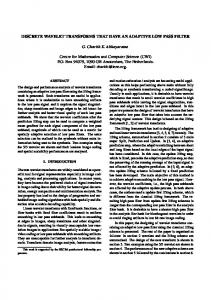
The above function is recursive where s and l represent integer constants for scaling and translation respectively. Scaling and translation will determine the type of wavelet that will be produced such as Wavelet Daubechies family (an example of one of them is shown in Fig. 1, i.e. Daubechies-6).

Fig. 1: Wavelet Analyser This wavelet analyser (WA) will be used to process every small signal that has been cut off earlier. To get a signal in varied resolutions, a scaling factor as shown below will be used [2][4]: W (x) =

N −2

∑

k = −1

( − 1) k c k + 1 Φ ( 2 x + k )

84

(2)

VHDL Development of a Discrete Wavelet Transformation

Φ , and ck is a wavelet coefficient.

where W(x) is a scaling function for wavelet analyser

To make the process

runs smoothly by using this scaling factor, the coefficient will have to meet the following linear and quadratic requirements: N −1

∑c

k

=2

k =0 N −1

∑c c

k k + 2l

k =0

(3)

= 2δ l , 0

(4)

where

δ is a delta function and l is the location index for the wavelet.

2.0

DISCRETE WAVELET TRANSFORM

Discrete wavelet transformation (DWT) is a method that uses WA, where it will translate and scale the particular WA. In DWT, the WA must be in discrete form as shown below:

φ ( x) =

M −1

∑ c φ (2 x − k )

(5)

k

k =0

where an additional range is determined by a positive value of M and C is a class of wavelet. The conditions for the coefficients are the same as in functions (3) and (4) respectively. Formula (5) is orthogonal by its own translation because it meets this requirement

∫ φ ( x)φ ( x − k )dx = 0 .

has to be orthogonal with its own translation. function

This formula also meets the second requirement that it

The second requirement i.e.

ϕ can be given as follows:

∫ ϕ ( x)ϕ (2 x − k )dx = 0 , where

ϕ ( x ) = ∑ (−1) k c1− kφ (2 x − k )

(6)

k

In DWT implementation, the Pyramid Algorithm [5] as shown in Fig. 2, is used. The usage of this algorithm follows one condition, i.e. the signal size must be a factor of 2, where t[n] and r[n] are highpass and lowpass functions respectively. X[n]

t[n]

r[n]

2

2

t[n]

r[n]

2

2

t[n]

r[n]

2

2

Fig. 2: Pyramid Algorithm Both functions can be given below [5]: ai =

bi =

1 2

N

∑c j =1

2i − j +1

fj

1 N ∑ (−1) j+1 c j+2−2i f j 2 j =1

85

N 2 N i =1,…., 2

i =1,….,

(7)

(8)

Razak and Yaacob

All the theories and functions that have been discussed earlier will be translated into programming code in MATLABTM and simulated to get the result.

3.0

DEVELOPMENT PHASES

As mentioned earlier, the programming code in MATLABTM is simulated and before one can proceed to program in MATLABTM, one has to determine all the related algorithms that will meet the theories and formulae. The result of the simulation process will be used for verification in a later SYNOPSYSTM process. This is to ensure the simulation result from SYNOPSYSTM is just as accurate.

4.0

MATLABTM SIMULATION

In this phase, all the processes that make a DWT are divided into small units relevant to the existing sub-processes. One of the algorithms that has been developed is shown below: 1. Flag = 0 2. Calling function get_h to get highpass coefficient form lowpass coefficient 3. while data size >= 2 3.1. setting new highpass and lowpass coefficient 3.2. if flag = 0 then 3.2.1 for I := 0 to (data size/2) do 3.2.1.1 calling lowpass, put result into array d. 3.2.1.2 calling highpass, put result into array h. 3.2.1.3 copy elements in d to array temp 3.2.1.4 set Flag = 1 3.2.2 end for. 3.2.3 copy elements in h to final array w in descending order. 3.3.else 3.3.1 repeat process 3.2.1.1 and 3.2.1.2 but input for both lowpass and highpass is form array temp 3.3.2 do initialization to array temp. 3.3.3 repeat process 3.2.1.3. 3.3.4 repeat process 3.2.3 to get next output of highpass 3..4. end if. 3.5. Data Size = ( Data Size /2) 4. end while. 5. end.

The following data are used in the simulation exercise that represents one-dimensional data: Input X = [0.1708,0.5724,0.0314,0.8033,0.1000,0.1011, 0.1111, 0.9801,0.9999,0.3311,0.8900,0.1231, 0.7651,0.0001,0.5555,0.9999]

The output data after the decomposition simulation are shown below in Table 1. To check that the decomposition has completed the correct processing of the data, the processed data will have to be built back to produce the original data. Table 2 below shows the output data that has been produced by inversion of the lowpass filter process.

86

VHDL Development of a Discrete Wavelet Transformation

Table 1: The decomposition result of DWT Steps

I

II

III

IV

V

W(1)

-

-

-

-

1.8837

W(2)

-

-

-

-0.3598

-0.3598

W(3)

-

-

0.2819

0.2819

0.2819

W(4)

-

-

0.5240

0.5240

0.5240

W(5)

-

0.1479

0.1479

0.1479

0.1479

W(6)

-

0.3511

0.3511

0.3511

0.3511

W(7)

-

0.5669

0.5669

0.5669

0.5669

W(8)

-

0.1852

0.1852

0.1852

0.1852

W(9)

0.0824

0.0824

0.0824

0.0824

0.0824

W(10)

-0.0123

-0.0123

-0.0123

-0.0123

-0.0123

W(11)

-0.5533

-0.5533

-0.5533

-0.5533

-0.5533

W(12)

-0.5037

-0.5037

-0.5037

-0.5037

-0.5037

W(13)

-0.1743

-0.1743

-0.1743

-0.1743

-0.1743

W(14)

0.6460

0.6460

0.6460

0.6460

0.6460

W(15)

0.3325

0.3325

0.3325

0.3325

0.3325

W(16)

0.3859

0.3859

0.3859

0.3859

0.3859

Table 2: Result data of Lowpass Filter Inversion Steps

I

II

III

IV

D_INV(1)

1.3320

0.7840

0.6628

0.6343

D_INV(2)

1.3320

1.1414

0.2718

0.2833

D_INV(3)

1.0997

0.3900

0.2609

D_INV(4)

0.7423

0.9790

0.4991

D_INV(5)

1.0227

0.3790

D_INV(6)

0.6133

-0.0239

D_INV(7)

0.5884

0.1586

D_INV(8)

0.7999

0.8820

D_INV(9)

0.9929

D_INV(10)

0.5946

D_INV(11)

0.4963

D_INV(12)

0.5145

D_INV(13)

0.4263

D_INV(14)

0.3360

D_INV(15)

0.4190

D_INV(16)

0.6820

Table 3 and Table 4 show the resulting data after inversion of the highpass filter process and the reconstructed data as a result of addition of the two results from the inversion of both highpass and lowpass processes.

87

Razak and Yaacob

Table 3: Result data of Highpass Filter Inversion Steps

I

II

III

IV

H_INV(1)

0.2544

-0.3799

-0.2393

-0.4653

H_INV(2)

-0.2544

0.2098

0.4087

0.2891

H_INV(3)

-0.1900

-0.4009

-0.2295

H_INV(4)

0.3600

0.2313

0.3024

H_INV(5)

-0.1330

-0.2790

H_INV(6)

0.0889

0.1250

H_INV(7)

-0.1114

-0.0475

H_INV(8)

0.1557

0.0981

H_INV(9)

0.0070

H_INV(10)

-0.2635

H_INV(11)

0.3937

H_INV(12)

-0.3914

H_INV(13)

0.3388

H_INV(14)

-0.3359

H_INV(15)

0.1365

H_INV(16)

0.3179

Table 4: Reconstructed data compared to the original data No

H_INV

D_INV

H_INV + D_INV

Original Data

1.

-0.4653

0.6343

0.1690

0.1708

2.

0.2891

0.2833

0.5724

0.5724

3.

-0.2295

0.2609

0.0314

0.0314

4.

0.3024

0.4991

0.8015

0.8015

5.

-0.2790

0.3790

0.1000

0.1000

6.

0.1250

-0.0239

0.0101

0.0101

7.

-0.0475

0.1586

0.1111

0.1111

8.

0.0981

0.8820

0.9801

0.9801

9.

0.0070

0.9929

0.9999

0.9999

10.

-0.2635

0.5946

0.3311

0.3311

11.

0.3937

0.4963

0.8900

0.8900

12.

-0.3914

0.5145

0.1231

0.1231

13.

0.3388

0.4263

0.7651

0.7651

14.

-0.3359

0.3360

0.0001

0.0001

15.

0.1365

0.4190

0.5555

0.5555

16.

0.3179

0.6820

0.9999

0.9999

Table 4 shows that the reconstructed data is matched to the original data and explains that all the algorithms and formulae used in this process were accurately designed. All the output data will be used in the next simulation process using SYNOPSYSTM tools.

88

VHDL Development of a Discrete Wavelet Transformation

5.0

SYNOPSYSTM SIMULATION

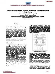
In this phase, all the programming code that were developed using MATLABTM are translated into the VHDL programming code. The new thing in this phase is the format of the data. The floating point format, i.e. IEEE 754, is being used. The architecture from the previous phase will be divided into smaller units and every function of the unit will be interconnected with each other. To get the accuracy in processing, an entity (as mentioned earlier) that controls all the flow of data is developed. Interconnection between entities is shown in Fig. 3. The coordination of data is also included in the figure. ACTUAL COEFF MEMORY

WORK COEFF MEMORY

TEMP WORK MEMORY

ACTUAL INPUT MEMORY

WORK INPUT MEMORY

BUS SELECTOR RESULTMEMORY

ACCUMULATOR

ADDER

LATCH_1

CONTROLLER

MULTIPLIER

LATCH_2

TEMP RESULT MEMORY

RESULR BUFFER

Fig. 3: DWT block diagram with data coordination The following are the result of the simulation and based on this result, it is shown that the algorithm described earlier delivered the accurate process successfully. In Table 5, the results respectively from MATLABTM and SYNOPSYSTM are in the floating-point format. These results are translated into decimal numbers so that they can be compared to the previous result in Table 1. It shows that these results match the result of decomposition and concludes that all functions in VHDL code were successfully developed.

89

Razak and Yaacob

Table 5: Simulation result of MATLABTM compared to SYNOPSYSTM

6.0

No

MATLAB result simulation (Hexadecimal)

SYNOPSYS result simulation (Hexadecimal)

Output data in Decimal

1.

3F711D14

3FF1174A

1.883523

2.

BEB837B4

BEB821D8

-0.359633

3.

3E905530

3E906C86

0.282078

4.

3F0624DC

3F062C50

0.524114

5.

3E177318

3E178F8A

0.148008

6.

3E013C360

3EB3D888

0.351261

7.

3F11205A

3F1122C4

0.566937

8.

3E3DA510

3E3DBAC5

0.185283

9.

3DA8C150

3DA8D808

0.082443

10.

BC498580

BC481330

-0.012212

11.

BF0DA512

BF0DA0E0

-0.553236

12.

BF0DF27C

BF00EA62

-0.503576

13.

BE327BB0

BE3253E4

-0.174148

14.

3F256042

3F2565C8

0.646084

15.

3EAA3070

3EAA477E

0.332577

16.

3EC594AC

3EC59F2A

0.385980

SYNTHESIS OF DWT

After the result has been put through the verification process, the synthesis process is carried out. In this phase, the gate logic diagram as shown in Fig. 4 has been successfully produced. It shows that the chosen algorithm has met the requirements of the design process.

7.0

CONCLUSION

The result from the simulation has paved the way for more experiments and trials to produce DWT in a physical chip. Up to this point, all the preparations to proceed to the next development are currently taking place. The next target will be to fabricate the design in an FPGA chip and to test the performance of the chip against the design requirements.

REFERENCES [1]

I. Daubechies, “Where Do Wavelets Come From? – A Personal Point of View”, in Proceedings of The IEEE, Vol. 84, No. 4, April 1996, pp. 510 –513.

[2]

A. Grasp, “ An Introduction to Wavelets”. IEEE Computational Science and Engineering, Vol.2, No.2, 1995, pp. 2.

[3]

Robi Polikar, “Wavelet Tutorial,” http://www.public.iastate.edu/%7erpolikar/WAVELETS/WTpart2.html, Dept. of Electrical and Computer Engineering, Iowa State University, June 1996.

[4]

M. A. Coffey, D. M. Etter, “Image Coding with The Wavelet Transform”. IEEE Symposium Circuit and System, Vol. 2, 1995, pp. 1110-1113.

[5]

S. Mallat, “A Theory for Multiresolution Signal Decompositions, the Wavelet Representation”. IEEE Trans. Pattern Analysis and Machine Intelligence, Vol. 2, 1989, pp. 674-693.

90

VHDL Development of a Discrete Wavelet Transformation

Fig. 4: Gate Logic Diagram

BIOGRAPHY Zaidi Razak obtained his Master of Computer Science from the University of Malaya in 2000. Currently he is a lecturer at the Faculty of Computer Science and Information Technology. His research areas include computer architecture, image processing and chip design. His current research is in image recognition of JAWI character alphabets.

91

Razak and Yaacob

Mashkuri Hj. Yaacob is currently a Professor of Computer Science and the Deputy Vice Chancellor (Academic Affairs) of the University of Malaya. He holds a PhD degree in Computer Engineering from the Victoria University of Manchester, United Kingdom. He is a Fellow of IEE, UK and a Fellow of the Malaysian Academy of Science. He has served the University for over 26 years and has held several academic and administrative positions. His current research areas are in computer architecture, computer networks and VLSI chip design.

92