Development of VHDL Model for Fixed-Point Discrete Wavelet Transform
Recommend Documents
This paper describes the development process of a discrete wavelet ... Scaling and translation will determine the type of wavelet that will be produced such as ...
Research Scholar, Jain University,. Bangalore. ..... A.C.Nuthan, M.S.Naveen Kumar, Shivanand S Gornale and Basavanna, âDevelopment of. Randomized ...
in performance. Keywords Discrete Wavelet Transform, Watermarking; Noise Attack, Salt and Pepper Noise, Compression, Bit Ma- ... Published online at http://journal.sapub.org/ajbe. Copyright ..... distortion-free image as reference. SSIM is ...
Abstractâ The use of discrete wavelet for image compression and a model of the scheme of verification of parallelizing the compression have been presented in ...
Surampalem, Kakinada. no matter how unbreakable will arouse suspicion, and may in themselves be incriminating in countries where encryption is illegal.
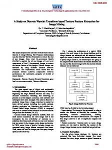
Abstract: This paper deals with using discrete wavelet transform derived features
used for digital image texture analysis. Wavelets appear to be a suitable tool for ...
an application of discrete wavelet transform (WT) and complex wavelet transform
(CWT) in image processing problem such as hybrid skeletonization.
Multimedia 3(2), 2001, 232â241. [4] Al-Haj A., Mohammad A. and Bata L., DWTâBased. Audio Watermarking, The International Arab Journal of. Information ...
The watermark is embedded using a secret or public key, making invisible changes to the ...... before compression, the empirical pdf of the correlations in the case for an incorrect watermark is ..... Published online 29, August, 2011 ... In order to
Abstract - This paper proposed an efficient image fusion algo- rithm for fusing medical images with the help of DWT & Spa- tial frequency techniques. The basic ...
Dr. Pauls Engineering College, Villupuram, India. E-mail:[email protected]@gmail.com. Abstract: Steganography is the art of hiding a secret ...
Keywords: Image compression, DWT, JPEG, GIF, PSNR, MSE,. Compression ratio. 1. Introduction. Image compression is important for many applications that.
Keywords: Image fusion, Discrete Wavelet Transform, Spatial. Frequency. I. INTRODUCTION. Image fusion is the process of combining relevant infor-.
Image up-sampling is found to be a very effective ... decomposition, the discrete wavelet transform (DWT) ... image to produce an intermediate result and then.
Jan 22, 2016 - Abstract. This paper highlights the potential of discrete wavelet transforms in the analysis and comparison of genomic sequences of ...
hiding the signal on his memory, sometime later invisible ink were the best method to hide .... [8] N. Provos and P. Honeyman, âHide and seek: An introduction to ...
Jul 12, 2002 - Delft University of Technology. Faculty of Information Technology and Systems. Type: Master's Thesis. Number of pages: 67. Date: 12 July ...
ABSTRACT: Power system transient (PST) disturbances occur for few cycles, which are very difficult to ..... http://mcct.quest.edu.pk/submission.html. [7]. Lachman ...
of music is presented. ... Wavelets for audio and especially music have been ..... "cure.plot". 0. 5. 10. 15. 20. 25. 30. 40. 60. 80. 100. 120. 140. 160. "bartok.plot". 0.
Summary. The image de-noising naturally corrupted by noise is a classical problem in the field of signal or image processing. Additive random noise can easily ...
by hiding multiple copies of the same data in the cover image using bit ... enhancement in the visual and statistical invisibility of hidden information after data recovery that supports ... via computer networks and conveniently processed for que-.
this work is to define the optimal wavelet function to use in DWT decomposi- ... Keywordsâbaseline drift, denoising, disrete wavelet transform, ECG signal,.
components of level 2 decomposed images to extract the texture ... that are natural in the images, color, shape and texture. ... Available [email protected].
Broadly speaking, the wavelet transform of a function consists of a coarse overall ... synopsis that comprises a select small collection of wavelet coefficients.
Development of VHDL Model for Fixed-Point Discrete Wavelet Transform
Abstractâ The wavelet transform is an efficient technique for multi-resolution analysis of non-stationary and fast transient signals. For this reason, wavelet ...
International Conference on Computer and Communication Engineering (ICCCE 2012), 3-5 July 2012, Kuala Lumpur, Malaysia
Development of VHDL Model for Fixed-Point Discrete Wavelet Transform Md. Rezwanul Ahsan, Muhammad Ibn Ibrahimy and Othman Omran Khalifa Department of Electrical and Computer Engineering, Faculty of Engineering International Islamic University Malaysia Kuala Lumpur 53100, Malaysia E-mail: [email protected]
However, wavelet transform can be the solution for the processing multi-resolution analysis of non-stationary and fast transient signals. Working on digital signal processing Stephane Mallat [2] provided a new contribution to wavelet theory by connecting the term filters with mirror symmetry, the pyramid algorithm and orthonormal wavelet basis. Yves Meyer [3] constructed a continuously differentiable wavelet lacking and finally, Ingrid Daubechies [4] managed to add to Haar's [5] work by constructing various families of orthonormal wavelet bases. The WT has many similarities with STFT but is basically different in its basis function called wavelets which are not of fixed length. Its time-frequency resolution plane provides good time localization at high frequencies and improved frequency discrimination at low frequencies [6]. Fig. 1 illustrates the comparison between time, frequency, timefrequency and wavelet representation of signal.
Abstract— The wavelet transform is an efficient technique for multi-resolution analysis of non-stationary and fast transient signals. For this reason, wavelet transform has been widely applied in signal analysis through processing, encoding, denoising and encrypting. The objective of this paper is to represent the development process of VHSIC (Very High Speed Integrated Circuit) Hardware Description Language (VHDL) based wavelet transform model. The VHDL model development is based on fixed-point arithmetic. A fixed-point number represents a number which has fixed number of digits after and before of the radix point and of real data type. Discrete Wavelet Transform (DWT) is a method that uses wavelet analyser in which case the signals composed into small pieces preserving both time and frequency properties. Out of the mother wavelet functions family, 2nd order of Daubechies (4-tap) has been widely used in denoising various types of biomedical signals. This research work involves with the VHDL modeling of Daubechies wavelet which is developed by Ingrid Daubechies. The functionality of VHDL model for DWT structure has been tested successfully and its performance level is in the satisfactory region (up to two decimal points of precision). Keywords- Discrete Wavelet Transform; Fixed-point Number; Hardware Description Language; Daubechies Wavelet; Signal Processing.
I.
INTRODUCTION
A wavelet is a waveform of effectively limited duration with an average value of zero. This is the basic form of analysis tool which has energy concentrated in time and utilized for the exploration of transient, non-stationary time-varying signals. In last two decades, the Wavelet Transform is found to be and efficient and popular technique in the area of signal processing. This is because of its ability to represent the signal in timefrequency domain, i.e. it can give the information related to both time and frequency simultaneously. The conventional Fourier Transform produces a discrete-time, discrete-frequency representation and it has very good frequency discrimination but poor time localization property. Additionally, the Fourier Transform only applicable to stationary signals. Davies and Reisman [1] find out that the Short-time Fourier Transform (STFT) distribution is unable to comply with four important properties required for time-frequency analysis of signal. The two properties are related to time and frequency marginals and the rest two are associated with time and frequency support.
Figure 1. Signal representation in different domain
In recent years, a considerable amount of interest can be observed for the implementation of wavelet transform architecture to facilitate real-time signal processing. For the demand of device portability and real-time applications, the wavelet architectures are implemented by targeting the physical Field Programmable Gate Array (FPGA) devices. The rapid changing technology introducing much more development to Electronic Design Automation (EDA) tools which in terns
appropriate choice of the mother wavelet function. Some of the popular standard families of the wavelet basic functions are Haar, Daubechies (db), Coeiflet (coef), Symmlet (sum), Morlet and Maxican Hat.
reduce the design cycle, complexity and valuable time to the programmer. However, the VHDL based algorithm development and design process not yet free from complexity and time consuming. Furthermore, it requires some sort of expertness and experience from hardware language field. There are insignificant related research works available because of quiet new and still developing field of research. However, some of the noticeable research in the development of hardware modelling of wavelet can be mentioned here.
Daubechies wavelets are families of wavelets whose inverse wavelet transforms are orthogonal. The numbers associated with the name refers to the number ‘N’ of coefficients. Each wavelet has vanishing/taping moments equal to half the number of coefficients. The number of vanishing moments decides the wavelet's ability for the representation of a signal. The wavelet transform using Daubechies wavelets results in progressively finer discrete samplings using recurrence relations. Every resolution scale is double that of the previous scale. For Daubechies wavelet transforms, the scaling signals and wavelets have slightly longer supports than Haar, i.e., they produce averages and diơerences using just a few more values from the signal. However, this slight change provides a tremendous improvement in the capabilities of these new transforms. Daubechies wavelets use overlapping windows, so high frequency coefficients spectrum reflects at high frequency changes. There are no explicit expressions for Daubechies compact support orthogonal wavelets and corresponding scaling functions. Table I presents the wavelet filter coefficients for Daubechies 4-taps wavelet for forward transform and inverse transform. Fig. 2 shows the corresponding scaling and wavelet functions. Generally, the discrete wavelet transform is implemented by using a hierarchical filter structure. Due to orthogonal property, the coefficients of Daubechies wavelet have relationship between the highpass and lowpass filters as shown in Equation (1).
In 1994, Vishwanath [7] have implemented a 3-level 1D DWT by using single processor with many processing units. The DWT architecture is implemented by applying the recursive pyramid algorithm based folding technique which is an old technique. Though this technique utilizes less hardware area, it requires a complex controller for adjusting the data flow from one level to the next. Moreover, the delay for the critical path could be high for higher orders. Mallat’s Fast Wavelet Transform (FWT) algorithm based implementation performed by Motra et. al [8]. Haar and Daubechies Wavelet Transform implemented and a very good comparison presented by Elfouly et. al. [9] on FPGA technology. Their design also utilized Finite Impulse Response (FIR) filter as building block and Lookup Table (LUT) for storing data. For forward and inverse transform operation, the parallel distributed arithmetic FIR filter used as basic building block whereas the data stores in look-up-table during operation. At the same time, Baganne et al. [10] have implemented Mallat's 3-level pyramid algorithm architecture directly with three cascaded DWT blocks. The architecture is of modular type; have low design complexity, low hardware latency and easily expandable to further levels of decomposition. However, it has large critical path delay and increased power dissipation due to performing unnecessary computations for down sampling.
H [ N − 1 − n] = (−1)n L[n]
This research involves with the development of VHDL model for a Daubechies 4-tap orthogonal architecture. A 16-bit fixed-point number system is used for VHDL modelling of DWT. The development process carried out by first designing the architecture in C++ programming platform. Afterwards, modular programming technique has been utilized to design the VHDL model. The advantage of modular programming is to reuse the hardware resources by performing similar task by executing same module. The development process, result and performance of the designed VHDL model are successfully verified by analyzing the outputs which are presented in synthesis and simulation section. II.
A. Wavelet Transform and its Architecture Wavelet transforms are of two types, Continuous Wavelet Transforms (CWT) and Discrete Wavelet Transforms (DWT). A wavelet transform decomposes a signal into shifted and scaled versions of the original wavelet. The DWT is performed by successive low-pass and high-pass filtering of the discrete time-domain. The resolution of a signal, which is a measure of the detail information in the signal, is determined by the filtering operations. On the other hand the scale is determined by up-sampling and down-sampling operations. The ability of DWT to extract features from the signal is dependent on the
Figure 2. Daubechies 4-tap Scaling and Wavelet function
For forward DWT, the signal is passed through a set of filter bank consisting of high pass filter for analyzing the high frequencies and low pass filter for analyzing the low frequencies. When the signal passed through filters a detail and approximation signal produced with same number of data points. At every level, the signal is down sampled by two and hence the output signals get half of the data points. The
453
point data and stored in memory as an array. When it has completed storing of all the input data, the output flag en_rd set to ‘high’ which acts as input flag for starting the operation of DWT_forward module. The number of data points and decomposition levels are also maintained in utilitipack package. When the 4 levels of forward transform has finished, it sets the en_fwd to high for starting the DWT_inverse module. The details coefficients from forward transform are then fed to inverse_DWT module. In this module, the approximation and details coefficients reconstructed to get back the signals. When inverse transform has finished, it set high for its output flag en_inv which is used as input flag for DisplayData module. Due to the constrain of pins for the I/O port of specific device family, DisplayData module is used for displaying the data. The output data for this module is in serial mode, hence it helps to save numbers of I/O pins.
decomposition of signal is continued with successive low frequency bands being decomposed termed as two-channel subband coder, developed by Mallat [2]. The following Fig. 3 presents a four level forward transform architecture.
Figure 3. Four level of forward DWT
Inverse wavelet transform is the reverse process of decomposition to reconstruct the signal. In this process, at every level the approximation and detail coefficients are upsampled by two and pass through inverse low pass and inverse high pass filters respectively. This process is iterated for four levels to reconstruct the signal. Fig. 4 gives the four levels of inverse wavelet transform based on the Fig. 3.
Figure 5. Top level entity DWT_FixedPt
Figure 4. Four level of DWT reconstruction
B. VHDL Modelling Scheme for DWT The structure of the db4 DWT has first modelled in C++ because the functionality and reliability can be easily verified there with faster response. Afterwards, the overall design has been modelled using VHDL. The EDA tool, Altera Quartus II version 9.1 SP2 web edition is used as the designing platform. The VHDL model comprises of structure, behavioural and physical version of the program. The EDA tool provides the facility to implement the synthesized and designed model into available FPGA device. The final VHDL model is developed by utilizing modular programming. The top entity DWT_FixedPt as shown in Fig. 5 is the main module to manage and control other components of it. The components as a module are Read_Data, DWT_forward, DWT_inverse and DataDisplay. The names of the components clarify their functions. The schematic diagram of the VHDL model is presented in Fig. 6. One of the property of the design is that it is generic (i.e., any number of input can be feed and multi-level decomposition can be performed) and computational number system based on 16-bit fixed-point. It should be noted that, number of input data must be integer multiple of 32 (25) to perform 4-level of transformation. An user defined package added namely utilitypack which defines the different data structure based on fixed-point, stores Daubechies forward and inverse coefficients, saves some constants and maintains a function to multiply two fixed-point numbers. The input data needs to convert in fixed-point before feeding to the model. The first module Read_Data collects the input 16-bit fixed
Figure 6. Schematic diagram of Discrete Wavelet Transform
C. Fixed-Point Number System The internal calculation of the designed VHDL model utilizes the IEEE proposed fixed-package [11], which has been added to the library. Fixed point number is of fixed exponent which is the reverse of floating point number which has varying exponent. No additional logic is required for the computation of exponents thus computational process gain significant speed. Moreover, fixed-point implementations required is less complex hardware which reduces considerable power consumption. For these reason, many hardware platforms (such as FPGAs) prefer fixed-point arithmetic where accuracy and precision is not important. The design cycle of VHDL model utilizes 16-bit fixed points with predefined format 6 down to -9. The MSB is the sign bit and 2’s complement is used for representing negative number.
454
performing simulation and other verification processes. Fig. 7 shows the Technology Map view of the designed VHDL model.
The conversion of fixed-point to fractional decimal is as below: 0010110101110011 (16 bit, positive) = 24+22+21+2-1++2-3+2-4+2-5+2-8+2-9 = 22.724609
The VHDL program model for DWT first tested for justifying the performance of forward and inverse transform. In that case, eight random data points of all possible combination used for two-level of decomposition. The output of VHDL model (only forward and inverse transform) and its comparison with C++ program output has outlined in the Table II and Table III. It shows that there is very slight difference which is because of number of input bit used. Use of higher number bit will give better precision but that will cost complex computation, bulky memory reservation as well as inefficient time consumption.
1010110101110011 (16 bit, negative) = - (0101001010001101) 2’s complement = - (25+23+20+2-2+2-6+2-7+2-9) = - 41.275391 D. Compilation and Functional Simulation After designing every VHDL module, it requires to compile separately for getting the better result and for debugging and testing perfection. If any fault found in the designed model, then it requires to modify the architecture and configuration to map the desired function of the module. However, modifying the architecture that contains the component instantiation statements requires recompilation of module which contains the architecture. All the modules for the designed model are compiled for the purpose of testing the Analysis and Synthesis check, Place & Route (Fitter) check Assembler check and Classic Timer Analyzer check by using the Quartus II software. Simulation is the most important part for VHDL based hardware modeling flow. It is also one of the most difficult part, not for the mechanism of the processes but because it needs to evaluate all possible processes and failure modes and also requires to test them carefully. The most systematic and thorough way to test the designed model is to apply all possible inputs or combination of inputs in an ascending binary sequence. The Quartus II software has the facility to create Vector Waveform File (.vwf) in the form of graphical waveforms that represents simulation inputs and outputs. To perform functional simulation, in this research, the inputs are given by using .vwf format through designing proper waveform for corresponding process modeling. A simulation summary report is generated after performing the compilation and functional simulation. As an empirical method of design verification, the simulation report presents that whether for a given set of inputs, the simulation model gives the desired output response or not and if there is any design error in the model. If the outputs from the simulation run satisfy the desired requirements then the designed model is considered as ok. Otherwise, it may require re-designed the design entry part again and perform continuous debugging process until the simulation run gives satisfactory output. III.
The output from Read_Data, DWT_forward and DWT_inverse are shown in Fig. 8 through vector waveform. After successful performance checking of the designed DWT model, 32 numbers of 16-bit fixed point data are fed to the model. The comparison between the VHDL model output and C++ output is presented in Table IV. The compilation summary of the designed model for 32 data points is shown in Fig. 9. The logic utilization is 35%, combinational ALUTs 10,840, total registers used 2961, total block memory bits 512 and total pins as I/O port 67. The output data from designed VHDL model and C++ program has also been presented as a comparison in Table IV. For forward transform, only approximation and details coefficients for different level present and in inverse transform the data points presents the constructed signal. It clearly shows that the VHDL model performs very well with very little lack of decimal precision points.
Figure 7. Technology map of the designed model
SYNTHESIS AND SIMULATION OF THE DESIGNED MODEL
The VHDL model for DWT has been analyzed, synthesized and simulated for the device StratixIII, chipset EP3SE50F780I4L. The Quartus II 9.1 software has in-built tools for performing these operations which will also generate gate level architecture namely Register Transfer Level (RTL) diagram for the designed model and all modules. Also Technology Map of the designed DWT model generated. RTL design shows flow of signals between hardware registers, and the logical operations performed on those signals. The RTL or Technology Map helps to check the design visually before
Figure 8. Vector waveform output from Designed VHDL model
455
REFERENCES [1]
M. R. Davies and S. S. Reisman, “Time Frequency Analysis of the Electromyogram During Fatigue,” in Proceedings of the 20th Annual Northeast Bioengineering Conference, USA, 1994, pp. 93–95. [2] S. Mallat, “A theory for multiresolution signal decomposition: the wavelet transform,” IEEE Trans. Pattern Anal. Machine Intell, vol. 11, no. 7, pp. 674–693, 1989. [3] Y. Meyer, Ondelettes et opérateurs: Ondelettes. Hermann, 1990. [4] I. Daubechies, “Orthonormal bases of compactly supported wavelets,” Communications on pure and applied mathematics, vol. 41, no. 7, pp. 909–996, 1988. [5] A. Haar, “Zur Theorie der orthogonalen Funktionensysteme.(Erste Mitteilung.),” Mathematische Annalen, vol. 69, pp. 331–371, 1910. [6] J. A. Crowe, “The wavelet transform and its application to biomedical signals,” in Time-Frequency Analysis of Biomedical Signals (Digest No. 1997/006), IEE Colloquium on, London, UK, 1997, pp. 2/1–2/3. [7] M. Vishwanath, “The recursive pyramid algorithm for the discrete wavelet transform,” IEEE Transactions on Signal Processing, vol. 42, no. 3, pp. 673–676, Mar. 1994. [8] A. S. Motra, P. K. Bora, and I. Chakrabarti, “An efficient hardware implementation of DWT and IDWT,” in TENCON 2003. Conference on Convergent Technologies for Asia-Pacific Region, 2003, vol. 1, pp. 95– 99. [9] F. H. Elfouly, M. I. Mahmoud, M. I. . Dessouky, and S. Deyab, “Comparison between Haar and Daubechies, Wavelet Transformations on FPGA Technology,” International Journal of Computer, Information, and Systems Science, and Engineering, vol. 2, no. 1, 2008. [10] A. Baganne, I. Bennour, M. Elmarzougui, R. Gaiech, and E. Martin, “A multi-level design flow for incorporating IP cores: case study of 1D wavelet IP integration,” in Design, Automation and Test in Europe Conference and Exhibition, 2003, 2003, pp. 250– 255 suppl. [11] D. Bishop, “Fixed point package user’s guide,” Packages and bodies for the IEEE 1076-2008 LRM.
Figure 9. Compilation Summary
IV.
CONCLUSION
The performance of VHDL model has been tested successfully with 32 numbers of fixed-point data. The comparison results in between VHDL and C++ model outpu shows the result in satisfactory region. The designed VHDL model of DWT architecture has achieved 2 decimal point precision. Higher precision can be obtained if 32-bit fixedpoint or IEEE floating point is used as arithmetic. However, in that case high speed processor with larger memory will be essential and it will then increase the complexity of computation. The future work may include using of floating point data and implement the designed model in physical FPGA device.