virtual machine placement algorithm for virtualized desktop infrastructure

Proceedings of IEEE CCIS2011

VIRTUAL MACHINE PLACEMENT ALGORITHM FOR VIRTUALIZED DESKTOP INFRASTRUCTURE Cao Le Thanh Man, Makoto Kayashima Yokohama Research Laboratory, Hitachi Ltd. 292, Yoshida-cho, Totsuka-ku, Yokohama-shi, Kanagawa-ken, Japan {lethanhman.cao.eq, makoto.kayashima.hh}@hitachi.com In a virtual machine infrastructure the resource of the servers can be effectively utilized by allocating virtual machines. For example, a study by Andrzej et al in [1] shows that by using a suitable allocation of virtual machines, up to 50% of the energy of the virtualization infrastructure can be saved. Thus, resource allocation in a virtualization infrastructure has attracted a great deal of research interest. According to the study by Beloglazov in [2], the virtual machine allocation problem can be divided into two stages. The first is the placement of virtual machines before the infrastructure starts to work [5, 6, and 8]. The second is the migration [7] of a virtual machine between servers if there is under- or over-utilization of the hardware resource when the infrastructure is working [2 and 4].

Abstract Finding optimal placement of virtual machines on numerous physical servers is one kind of binpacking problem, which is known as an NP-hard. We propose the use of a heuristic algorithm to solve this problem where the virtual machines play the roles of personal desktops. As we have found out that the changes in the amount of hardware resources required by a desktop often repeat a certain pattern, in the proposed algorithm, we uses the correlation between the patterns to find the group of desktops that are most suitable for sharing the same physical server. Simulation results show that the proposed algorithm can be used to reduce the number of physical servers required for hosting a certain number of virtual desktops. Keywords: Virtual desktop, infrastructure, Resource allocation

We focused on the virtual machine placement stage. This is important because, if the initial placement of virtual machines is not suitable, the number of servers increases and the number of migration on the second stage also increases. The number of servers should be kept as low as possible to reduce costs. Furthermore, the number of migrations of a virtual machine should be kept as low as possible to save the energy as well as minimize the traffic and service delay caused as a result of the migration period. However, finding the optimal placement of virtual machines on numerous physical servers is a kind of bin-packing problem, an NP-hard. This is also the case with a virtual desktop because the hardware resources required by a desktop change quickly over time because of the action of the users. The placement problem is thus much more difficult to solve.

Virtualization

1 Introduction To simplify the administration tasks of information systems, the platform virtualization technology has been used. Hardware resources of the servers can thus be shown as multiple logistical resources, which can then be shared with many machines running separately. Moreover, the virtual machines do not have a strong relationship to the hardware characteristic of the servers, so they can be easily transferred between servers. The platform virtualization technology has been widely used on Web and database servers. Recently, a new usage of this technology, the virtualization of desktops, has been deployed. The operating system of desktops is installed on virtual machines, which are located on a virtualization infrastructure in a data center, and the user remotely operates the desktops via thin clients. Virtualization of desktops enables data and applications to be centralized, and, thus, the cost of managing a PC is reduced and the risk of information leaks minimized.

We propose an approach for solving the problem of virtual desktop placement. The approach is called Pattern-based Virtual Desktop Allocation (PBA). As we have found that the desktops for office users often repeats some fix pattern because of the working style of the user, PBA deploys the patterns for virtual desktop placement. It is used to place the desktops of which the patterns have low correlation coefficient on the same servers. Thus, this approach provides the virtual desktops with sufficient hardware resources to perform at their

___________________________________ 978-1-61284-204-2/11/$26.00 ©2011 IEEE

best while keeping the number of physical servers as low as possible.

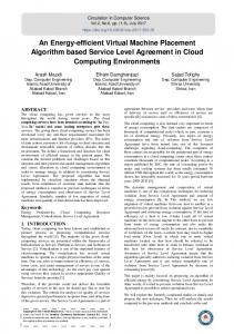
software. The autocorrelation of the CPU usage for 12 virtual desktops is shown in Figure 1. Collected data shows that for the entire desktop, the CPU usage has high autocorrelation when the lag is 24 hours. This means the CPU usage of a desktop almost repeats the same pattern every 24 hours (one day).

2 Related research The study by Bobroff et al in [5] proposes a general model for virtual machines resources placement, which is a generalization of the classical 0/1 Knapsack problem. The authors proposed that each virtual machine has a fixed the profit value and utilizes First Fit, Next Fit, and Best Fit to obtain the near highest profit. In [8] F. Hermenier et al has proposed the Best Fit and First Fit based algorithms. To save the electric consumption of the system, a Best Fit-based algorithm has been used in [2]. A study in [6] also uses the Best Fit-based algorithm on the predicted value of the resource consumed by the virtual machine. The common feature in existing algorithms is that they use one value, for example, the average value to express the amount of the resource that the virtual machine consumes. This is simple and effective when the resource does not change significantly during the time, such as a Web server of a database server. However, a the resources of a virtual desktop change significantly as a result of the action of the user, so expressing the amount by a fixed value is not suitable.

1 0.8 0.6 Autocorrelation

0.4 0.2 0 -0.2 -0.4 -0.6 0

4

8

12

16

20

24

28

32

36

40

44

48

52

56

60

64

68

72

76

80

84

Lag (Hours) Desktop 1 Desktop 5 Desktop 9

Desktop 2 Desktop 6 Desktop 10



Figure 1. Autocorrelation of CPU usage of virtual desktops Initial placement

Server groups VMM

VMM

VD 1

VMM

VD 2

VD3

Final placement

VMM

VM groups VD1

Placement

VD2

VD 3

VDn

䇯䇯䇯

VD 4

VD 2

VMM

SLA-based migration

䇯䇯䇯 VM resource utilization 100

60 40 20

VD n-1

100

80 60 40 20

80 60

VD 6

VD 䌮

40

0-2 2-4 4-6 6-8 8-10 10-12 12-14 12-16 16-18 18-20 20-22 22-24

0

ᤨ㑆Ꮺ

ᤨ㑆Ꮺ

ᤨ㑆Ꮺ

VMM

VD 4

VD 1 VMM

䇯䇯䇯

20

0-2 2-4 4-6 6-8 8-10 10-12 12-14 12-16 16-18 18-20 20-22 22-24

0 0-2 2-4 4-6 6-8 8-10 10-12 12-14 12-16 16-18 18-20 20-22 22-24

0

CPU೑↪₸

80

CPU೑↪₸

CPU೑↪₸

100

VD 3 VMM

SLA-based migration

䇯䇯䇯

SLA

Output

VD n-1

VM resource utilization

VD n VMM

VM: Virtual machine SLA: Service Level Agreement

3 Characteristic of virtual desktops

100

40 20

100

80 60 40 20

80 60 40 20 0 0-2 2-4 4-6 6-8 8-10 10-12 12-14 12-16 16-18 18-20 20-22 22-24

0 0-2 2-4 4-6 6-8 8-10 10-12 12-14 12-16 16-18 18-20 20-22 22-24

0

CPU೑↪₸

CPU೑↪₸

80 60

0-2 2-4 4-6 6-8 8-10 10-12 12-14 12-16 16-18 18-20 20-22 22-24

CPU೑↪₸

100

Input

ᤨ㑆Ꮺ

ᤨ㑆Ꮺ

ᤨ㑆Ꮺ

SLA

Figure 2. Overview of virtual desktop allocation

Resources that a virtual desktop requires are HDD access bandwidth, CPU processing power, a specific amount of memory and the network bandwidth. Among these, the network bandwidth is not a bottleneck for general office use because the NIC of a server is usually 1 or 10 Gbps and larger than the network path. The memory needs to be sufficient for the OS to work because a shortage significantly affects the performance of the OS. Therefore, we assume that the server only accept the virtual machine when is can allocate enough memory for the machine to work normally (usually 1 - 2 GB for an office user’s desktop). The HDD may be a bottleneck of a virtual server with many virtual machines running on it, but when it changes to SSD or a high-performance network attached storage, the bottleneck is cleared. Meanwhile, CPU resource is the one that needs to be considered because the virtual machines sharing the same CPU directly affect each other. Thus, we only focus on these resources when solving the problem of placement of virtual desktops.

We conclude that the CPU usage of virtual desktops of office users repeat almost the same pattern in a fixed period of time. In the experiments, the length of the pattern is one day. In other office environments, this length may be one week or one month because of the type of work of the users. Each pattern has a different max value and timing when it reaches the max value. This value depends on the habits, the work, and the period the users present at the office.

4 Proposed algorithm 4.1 Overview on virtual desktop allocation We illustrate two stages of virtual desktop (VD) allocation in Figure 2. The placement phase has the input including the server groups, VM groups, VM resource requirements, and the SLAs. The output of this phase is the initial placement of the virtual machine. The infrastructure starts to work with the initial placement. During the working time of the infrastructure, the migration may be done to protect the SLA. The migration may happen many times until the infrastructure stops working. The number of servers may increase because of the migration. When the systems stop the final number for servers required in the systems may differ from

We have monitored the CPU resource consumed by virtual desktops of a group of randomly selected office users in one week. The users remotely login and operate the virtual desktops. The main applications used are text editors, presentation materials editors, and schedule control

that needed in the initial placement. To reduce the cost of the infrastructure, the final number of servers in the final placement needs to be minimized. Also, the time of migration also needs to be reduced. The number of servers and the migration times is affected by the algorithm of migration and also by the initial placement.

The output of PBA is given by the following matrix.

Here, . PBA utilizes the following functions. Max_average_index(S): This function returns the index of the VD in the set S which has the largest average value of CPU usage. Min_correlation_index(F(t),S) ˖ This function returns the index of the VD in the set S of which the pattern has smallest correlation coefficient with F(t). Here F(t) is a pattern of CPU usage. Following is the details of PBA algorithm. It contains 7 steps. 1. Reset the output matrix

4.2 Proposed algorithm We named the proposed algorithm pattern-based virtual desktop allocation (PBA). The rationale of the approach is as follows. For each server, the PBA places as many virtual desktops as possible as long as the server meets the SLA requirements. After finishing placing the VDs on a server, PBA continue to place the VDs on the next server. This task repeats until all the VDs are placed. The task of placement of VDs on one server is as follows. First, PBA places a VD that has the biggest average CPU usage among the VD that is not assigned. The PBA places the VD that has the CPU usage pattern with smallest correlation coefficient with the VDs that has already been placed in the server. Thus, the VDs placed in the same server have low correlation coefficient with each others, so the opportunity for CPU contention in the servers is low. The details of the PBA algorithm are as follows.

( 2. Select a server as the first server. 3.

Place the first VD to the server

)

.

The first VD that is placed in the server is the one has largest average CPU usage among the VDs that is not placed in any servers. This means that to the server PBA place virtual desktop where = Max_average_index

The input of PBA algorithm is as follows: Let V the set of all virtual desktops that need to be placed.

㧔{

|

=1}㧕

, then the output matrix is updated. .

Here, N is the number of the virtual desktop in V, and W is the set of physical servers available for the placement of the virtual desktops in V. The number for servers is M. Here, we suppose that M is large enough for the placement of virtual desktops in V. For each server cores is

Here, we suppose that for each server, at least one VD can be placed without the violation of SLA. 4. Check for available VD for assigning to server Create the subset R from the VDs that are not allocated to any servers. This is the set of VDs that . can be placed in server R=

in W, the number of the CPU

. We suppose that the entire cores have

{{

the same power. For each virtual desktop in V, . expresses the CPU usage is shown by the percentage of one CPU core that where T consumes at the time t. Here, t . is the length of CPU usage pattern of desktop is . We define The average value of function SLA() as follow. Even when all the VDs in the set S are placed in the server , the server still meets the SLA agreements then is True; otherwise it is False. The SLA() function is decided as follows:

|

=1}

|

Here, L is the set of VDs that are already assigned . to server { | =1} When R is an empty set, there are no VDs . In this case, the available for assigning to PBA algorithm jumps to Step 6. 5. Place the second and later VD to server From the subset R, the following and placed in server

Here, S is a subset of V. ,where

. We have

is selected

= Min_correlation_index( 6.

the function expressed in Equation 1. In this is the maximum value of equation, parameter , the CPU usage pattern of the virtual desktop is the time that the desktop reaches the is the length of the period maximum value and that the desktop mainly used the CPU. We suppose that the real value of CPU of each VDs varies within D% from the average value. In the following simulations, the value of D% is set to 10% by default.

)

Check if there are VDs that have not placed yet.

If the following set is empty, then PBA stops. } When Q is not empty, the algorithm continues to step 7. 7.

Assigning VDs to the next server

˄1˅

Final server number

Here,

.

160

1

140

0.9 0.8

120

0.7

100

0.6

80

0.5

60

0.4 0.3

40

0.2

20

0.1 0

0

The PBA algorithm cannot obtain the optimal results for the problem of placement of N virtual desktops to M servers. However, for each server, PBA manages to place VDs with different CPU usage patterns. Therefore, the VDs do not conflict with each other. Thus, one server can, without violating the SLA agreements, contain more VDs. The algorithm is to be more effective in the environment where the patterns of the VDs are far different to each other.

VDI migration ratio

Jump to step 3. The seven steps above mean that the index of server j is gradually increased. In step 5, if Q is empty, PBA algorithm finishes because all VDs that needs to be placed are all placed. At this time, the value of j is the number of servers required for initial placement. The placement result is in matrix .

100

200

300

400

500

Number of virtual desktops FF_ave (Final server number)

FF_max (Final server number)

PBA (Final server number)

FF_ave (VD migration ratio)

FF_max (VD migration ratio)

PBA (VD migration ratio)

Figure 3.Number of servers and VD migration ratio 5.2 VD placement results when VD numbers change First, with a given number of virtual desktops, we examined the number of servers that each algorithms needs to place the virtual desktops. The number of migration during the operation time is also considered. The final number of servers needed to place the virtual machines when the placement algorithm are FF-ave ˈ FF-max, and PBA are shown in Figure 3. The number of VD was 100, 200, 300, 400, and 500. The number of servers here is not the initial but in the final placement, after a rotation of migration based on the SLA agreements. The VDs migration ratio is the ratio between the number of entire VDs that are placed and the number of VD migrations. From Figure 7, we see that the percentage of servers when PBA is used is always 9%which is 20% smaller than that in FF-ave and FF-max, respectively. Moreover, the VD migration ratio of FF-max is the lowest. This result is easy to understand because FF-max uses the maximum value of CPU usage. In contract, FF-ave introduces a high value of VD migration ratio (36%). Meanwhile, the VD migration ratio of PBA is approximately 5%, higher than that of FF-ave but much lower than that of FF-min.

5 Evaluation results We implemented and evaluated the proposed virtual desktop placement algorithm in a simulation environment. We have built a simulation environment using the Perl Programming Language. 5.1 Simulation settings We compared PBA with two First Fit [9] algorithms: FF-ave and FF-max. FF-ave is the First Fit algorithm applied to the average value of the CPU usage. FF-max is the First Fit algorithm applied to the max value of the CPU usage. An algorithm similar to FF-max is proposed in [6], and PBA is the proposed algorithm explained in Section 3. We used a simple FF-ave based algorithm for migration algorithm. When a virtual desktop needs to find a destination server to migrate to, the FF-ave algorithm was used to determine the destination server. In the following simulations, the SLA agreements were supposed to be “the average of CPU usage in 2 hours does not exceed 85%”. The number of CPU cores in the servers is supposed to be 2. This means , To create the patterns of CPU usage of the virtual desktops, we used the Gaussian distribution with

5.3 VD placement results when patterns errors change

As explained in Section 4, PBA bases on the information of the CPU usage patterns of the virtual desktops. Therefore, here we examined the performance of the algorithms when the value of D%, the relative error of the CPU usage varies. In the next simulation, we changed the value of D% from 10 to 30, 50, and 100 consequently and checked the number of servers in the final placement as well as the migration ratio. The number of VDs was set to 300. We did 10 simulations for each algorithm and collected the average values. The simulation results are shown in Figure 4. When D% increases, the VD migration ratio increases in all the algorithms. However, when D% is 100%, the number of servers when using PBA is still 6%, 16% lower than that when using FF-min, FF-max, respectively.

PBA. However, PBA keeps its VD migration ratio as low as 4% when the percentage of the server is only 51% and 13% of that of FF-max and FF-min, respectively.

6 Conclusion and future work We have proposed the use of an algorithm, PBA, that leverages the CPU usage patterns of the virtual desktops when placing the virtual desktops to the physical servers. With this algorithm, the number of servers required for placing virtual desktops is reduced. Furthermore, the number of virtual desktops that need to be migrated during the use of the virtualization infrastructure is also lower in comparison with First Fit, a common algorithm for solving the pin-packing problem. In our future work, we will evaluate the PBA algorithm in a real network environment.

1

120

0.9

References

0.8 0.7

80

0.6 0.5

60

0.4 40

0.3

VD migration ratio

Final server number

100

[1] Andrzej Kochut, “Power and Performance Modeling of Virtualized Desktop Systems”, in Proceedings of MASCOT 2009 [2] Beloglazov, Anton Buyya and Rajkumar, “Energy Efficient Resource Management in Virtualized Cloud Data Centers”, in Proceedings of the 10th IEEE/ACM CCGrid, 2010 [3] Yazir, Y.O., Matthews, C. et al., “Dynamic Resource Allocation in Computing Clouds Using Distributed Multiple Criteria Decision Analysis”, in Proceedings of the 3rd IEEE CLOUD, 2010 [4] A. Kochut and K. Beaty, “On Strategies for Dynamic Resource Management in Virtualized Server Environments”, in Proceedings of the 15th MASCOTS, 2007 [5] Paolo Campegiani and Francesco Lo Presti,” A General Model for Virtual Machines Resources Allocation in Multi-tier Distributed Systems”, in Proc. of the 5th ICAS, 2009 [6] Bobroff. N., Kochut. A. and Beaty. K., “Dynamic Placement of Virtual Machines for Managing SLA Violations”, in Proceedings of the 10th IFIP/IEEE IM, 2007 [7] Anthony Nocentino and Paul M. Ruth, “Toward Dependency-Aware Live Virtual Machine Migration”, in Proceedings of the 3rd VTDC, 2009 [8] F. Hermenier, et al., “Entropy: A Consolidation Manager for Clusters”, in Proceedings of ACM SIGPLAN/SIGOPS VEE, 2009 [9] E.G.C.Jr., M.R.Garey and D.S.Johnson. “Algorithms for Bin Packing: A Surveyā, Approximation algorithms for NP-hard problems, pages 46-93, 1996

0.2

20

0.1 0

0 10

20

50

100

Relative error of patterns(%) FF_ave (Final server number)






Figure 4. Effect of relative error (D%) 1

250

0.9 Final server number

0.7 0.6

150

0.5 100

0.4 0.3

VD migration ratio

0.8

200

0.2

50

0.1 0

0 100

200

300

400

500

Number of virtual desktops FF_ave (Final server number)






Figure 5. Effect of CPU usage 5.4 VD placement results when patterns errors change Finally, we investigated the VD placement results when the CPU usage patterns change. We set the of in Equation 1 value of the parameter to a smaller range as follows: This means, the distribution of the patterns became smaller. Here, the time when the virtual desktops use the CPU shortened. When the CPU usage patterns have a smaller distribution, the result in Subsection 5.2 changes to that shown in Figure 5 In this case, the VD migration ratio of FF-ave is as high as 47% and the number of servers when FFmax is used is as high as twice that of FF-ave and