the blobs in the scene. The principal angles computed during vector quantization along with other cues of the object are used for classifica- tion of detected ...
Vision-based Monitoring of Intersections Harini Veeraraghavan, Osama Masoud, Nikolaos Papanikolopoulos {harini, masoud, npapas}@cs.umn.edu Artificial Intelligence, Vision and Robotics Lab Department of Computer Science and Engineering University of Minnesota
Abstract— The goal of this project is to develop a passive vision-based sensing system. The system will be capable of monitoring an intersection by observing the vehicle and pedestrian flow, and predicting situations that might give rise to accidents. A single camera looking at an intersection from an arbitrary position is used. However, for extended applications, multiple cameras will be needed. Some of the key elements are camera calibration, motion tracking, vehicle classification, and situations giving rise to collisions. In this paper, we focus on motion tracking. Motion segmentation is performed using an adaptive background model that models each pixel as a mixture of Gaussians. The method used is similar to the method of Stauffer et al. for motion segmentation. Tracking of objects is performed by computing the overlap between oriented bounding boxes. The oriented boxes are computed by vector quantization of the blobs in the scene. The principal angles computed during vector quantization along with other cues of the object are used for classification of detected entities into vehicles and pedestrians. Keywords– Motion segmentation, principal component analysis, tracking, scene monitoring.
1
Introduction
The goal of this project is to develop a system that can track traffic objects in real-time in order to detect situations giving rise to accidents. This would involve using the trajectories of the objects over time to predict future trajectories and then analysing these trajectories. Standard background subtraction methods like time averaging of images or inter-frame differencing are not very robust in situations with many slow moving objects or in scenes where the majority of the background is covered most of the time. ∗ author
to whom all correspondence should be sent.
∗
Rosin et al. [3] perform background detection by using a median filter for each pixel. The difference images are then thresholded using automatically generated thresholds. Pfinder [8] uses a single Gaussian for the background and multiple statistical models for the foreground objects. However, the method is only suitable for relatively static scenes. Several methods exist for tracking objects in scenes. Coifman et al. [4] employ a feature based tracking method in which corner points of vehicles are tracked over time. The feature points are grouped based on the common motion constraint. Heisele et al. [5] track moving objects in colored image sequences by tracking the color clusters of the objects. Other tracking methods involve active contour based tracking, 3-D model based tracking, and region tracking. Motion segmentation is the first step in detecting the objects in a scene. We use a robust adaptive background segmentation method similar to the method of Stauffer et al. [6, 7]. This segmentation is very robust to variations in the scene due to changes in illumination, camera noise, moving tree leaves, slow moving objects, etc. The individual regions are extracted using connected components extraction. The amount of overlap between bounding boxes from two different frames is used to determine the relation between the respective regions. In contrast to horizontally aligned bounding boxes, oriented bounding boxes provide tighter fit to objects irrespective of their orientation with respect to the image axis. Thus, the oriented boxes are used to model the blobs. They are computed by vector quantization of each blob as explained in the following sections. Region tracking is used for tracking objects over time. Bounding boxes of the blobs are used to model the traffic objects. The tracking methodology used is similar to Masoud’s pedestrian tracker [2]. The eigenvectors along with the aspect ratio, velocity, and size are used for classifying the
blobs. Incident detection is done based on the proximity of traffic objects with respect to one another. Although our goal is to predict future incidents, our current focus in to look for imminent collisions. The paper is arranged as follows: The motion segmentation method is discussed in Section 2. Section 3 describes a vector quantization method for computing the oriented bounding boxes. The tracking method is discussed in Section 4. Scene monitoring, camera calibration, and the incident detection visualization tool are described in Section 6. Results, future work and conclusions are discussed in Sections 7, 8, and 9.
2
Motion Segmentation
Standard adaptive background estimation methods such as time averaging of the frames provide an approximate representation of the background scene except for parts of the scene undergoing motion. These methods perform poorly on scenes with a large amount of clutter, slow moving objects, etc. The recovered foreground often exhibits “ghosts” or trails behind a moving object. One example where this could be a problem is a scene with a platoon of slowly moving vehicles. In a case like this, all or most of the objects are merged into one, resulting in tracking errors. An example of the ghosting effect is shown in the Figure 1.
2.1
Stauffer’s Method for Adaptive Background Model
In [7], each pixel is modeled as a pixel process; each process consists of a mixture of k adaptive Gaussian distributions. The distributions with least variance and maximum weight are isolated as the background. The probability that a pixel of a particular distribution will occur at a time t is determined by P (Xt ) =
k X
ωi,t ∗ η(Xt |µi,t , Σi,t )
where ωi,t is the estimate of the weight of the ith Gaussian in the mixture at time t and µi,t and Σi,t are its mean and covariance. The value of k is chosen based on the speed of the computation required and the available memory. Each pixel is compared to the existing distribution until a match is found. When no match is found, the least probable distribution is replaced by the recent distribution. The weights of all the distributions are then updated using ωk,t = (1 − α) ∗ ωk,t−1 + α ∗ Mk,t
2 σt2 = (1 − ρ)σt−1 + ρ(Xt − µt )T (Xt − µt )
(b) current image
Figure 1: Approximated background, current image, and segmented image.
(3) (4)
where ρ = α ∗ η(Xt |µk , σk ) is the learning factor for the current distributions. The Gaussians having the least variance and maximum weight form the background in the scene. In other words, the models with high ω/σ value correspond to the background.
2.2
(c) segmented image
(2)
where α is the learning rate and Mk,t is 1 for matched distribution, and 0 otherwise. µ and σ remain unchanged for unmatched distributions while they are updated for the matched distribution using µt = (1 − ρ)µt−1 + ρXt
(a) approximate background
(1)
i=1
Connected Components
The individual regions are extracted using a twopass connected region extraction method. A raster scan of the binarized image is performed in the first stage coding the image as runs. A run is a set of contiguous 10 s on a single scan-line. Each scanline is always assumed to begin with 00 s. During the second pass, the runs computed from the first stage are grouped along rows to form regions. Each region is assigned a unique label. Statistics such as
area, perimeter, centroid, length, breadth etc., are partially computed during the second pass. Other statistics that are computed include elongation, aspect ratio, and higher order moments of the blob.
3
Oriented Bounding Box Computation
The oriented bounding box for each blob is computed by using a method of Principal Component Analysis (PCA), called vector quantization. PCA is a method of reducing a large number of dependent variables p into a smaller set of independent variables t. The transformation of the dataset from
4
A single camera is used to provide input to the system. Bounding rectangles are used to model the vehicles and pedestrians in a scene. Each bounding box is associated with attributes such as position, area, elongation, velocity, pedestrian/vehicle flag, age etc. The pedestrian/vehicle flag indicates whether a blob is a pedestrian or a vehicle. The blobs are computed from motion segmentation and connected component extraction as explained in the previous Section 2. In a typical scene, blobs obtained from the above method do not always have one-to-one correspondence with pedestrians and vehicles. As a result, a many-to-many relationship is assumed between the blobs and the entities in the image. This relation is updated temporally based on the observed behavior of the blobs.
4.1
Figure 2: Horizontally aligned minimum bounding box vs. oriented bounding box. the original space to feature space consists of a rotation and translation where, rotation is given by the direction of first principal axis and translation is the centroid of the dataset. The covariance matrix for each blob is given as: � � M20 M11 (5) M11 M02 th
where, Mi,j is the (i, j) order moment of the blob. X (6) Mij = (x − x)i (y − y)j .
Tracking Methodology
Blob Tracking
The blob tracking method applied is similar to Masoud’s pedestrian tracker [2]. A set of blobs occuring in a frame i are related to the blobs occuring in the frame i − 1 using an undirected bipartite graph G(Vi , Ei ) where Vi = Bi ∪Bi−1 . Bi and Bi−1 are the sets of vertices associated with the blobs in frames i and i − 1 respectively. In each frame, the association of each new blob in the ith frame is sought with the blobs in the th (i − 1) frame. Thus, tracking is equivalent to constructing a new association graph for every new frame. With each frame, the blobs are allowed to split, merge, appear, and disappear. To simplify graph computation, the following constraints are imposed: Parent Constraint From one frame to another, a blob may not participate in a split and merge operation at the same time.
R
Diagonalizing M, gives M = ∆T D∆ (7) � � where ∆ = � v1 v�2 represents the eigenvectors e1 0 and D = represents the eigenvalues. If 0 e2 e1 > e2 , we choose v1 as the principal axis with elongation 2.e1 . The angle made by the principal axis with respect to the x-axis of the image is also computed from the vector. Similarly, v2 is chosen as the second principal axis with elongation 2.e2 . Figure 2 illustrates the difference between using a horizontally aligned bounding box and a box oriented and sized using this method.
Locality Constraint Two blobs i.e.,vertices, can be connected only if they have a bounding box overlap area which is at least half the size of the bounding box of the smaller blob. The graph computation is done in two steps. In the first step, a graph in which no node violates the locality constraint is constructed. This can be done easily by checking the overlap area of the bounding rectangles. Only rectangles having an overlap area at least more than the bounding box area of the smallest rectangle are related. There can be only one such graph. In the second step, one valid graph is computed by pruning the nodes not satisfying the parent structure constraint. There could be several
such valid graphs. Instead of enumerating several valid graphs and then picking the least cost graph as in [2], only one valid, dense graph is computed. Given a high frame rate and a good background subtraction method, very few blobs will undergo splitting and merging at the same time. Even in cases where the split and merge occurs, the heuristic relates the new blob to the parent with which it has maximum percentage overlap. As a result, the computed graph is fairly accurate. The graph re-computation is done only for those nodes that do not satisfy the parent structure constraint. Violation of the constraint takes place when either of the following occurs: (1) a given parent node has multiple children and one or more of them has more than one parent, or, (2) a parent has one child and the child has at least one parent which participates in a split operation. In any of the above cases, the algorithm computes the cost of node connection for a given parent-child pair and other parent-child pairs whose participation with respect to the given child node causes the violation. The cost of a parent-child connection is given by cost =
abs(P (A) − ΣNc C(A)) max(P (A), ΣNc C(A))
(8)
in the case of a split and cost =
abs(ΣNp P (A) − C(A)) max(ΣNp P (A), C(A))
(9)
in the case of a merge. P (A) is the area of parent, C(A) is the area of child, Nc is the number of children of a given parent and Np is the number of parents of a given child. The parent-child node having the least cost is allowed to keep the connection while the remaining connections are eliminated. The connection that results in least variation in size from one generation to the next (parent to child) is given the least cost. Those connections that result in maximum size variation across frames incur maximum costs. Thus, child nodes that do not have any parent node (e.g.,when a blob disappears and reappears etc.) will have a very high cost. The algorithm is not guaranteed to find the least cost optimal graph all the times. However, for our purposes the algorithm is fairly accurate and faster than using several iterations to enumerate a single graph.
4.2
Bounding Box Overlap Computation
Bounding box overlap computation is complicated due to the fact that the boxes are oriented
in arbitrary directions with respect to each other. Hence, overlap computation is done by considering the rectangles as polygons. Polygon clipping algorithms can be used for computing the overlap. Alternatively, we could use a simple two-step method. In the first step, overlaps between bounding rectangles formed by corner points of the two boxes are computed. This step is done just to eliminate unrelated blobs to save computation. In the next step, each corner point of a rectangle is considered with respect to the other rectangle and the number of points inside and outside the rectangle is found. These points are used to compute the intersecting points. The same step is repeated considering the points of the latter rectangle with respect to the former. After eliminating the redundant points, the polygon area is computed from the remaining points after reordering. This corresponds to the overlap area.
5
Classification
The principal axis angles estimated for computing the oriented bounding boxes in Section 3 are used along with certain other attributes of the blob to classify the blobs as vehicles or pedestrians. The tracked blobs inherit the same attribute as their parent blobs. The motivation for using principal component axis angles is that pedestrians generally appear as long thin blobs and the principal axis is generally 90◦ to the x-axis while the vehicles are generally wide blobs. Along with this, the size and the velocity of the blobs are used for classification. This method works as a good preliminary classifier in situations with minimal clutter and no shadows.
Figure 4: Objects classified as vehicles (v) or pedestrians (p).
6
Scene Monitoring
Apart from tracking, the system must be able to identify situations where probable collisions be-
(a) sunny
(b) sunny with clouds
(c) snow
Figure 3: Tracking sequence under different lighting conditions, (sunny, sunny with clouds, and snow). tween vehicles might occur. In order to accomplish this, the system needs the position, length, width, velocity, etc., of the vehicles in world coordinates. Moreover, the system needs to predict the future in order to predict incidents that might occur in the future. Currently, we only deal with incident detection up to the current frame. We do this by detecting if the distance between any two vehicle oriented bounding boxes is less than a threshold. The results are presented visually using an incident detection visualization tool that we developed. The tool is a graphical user interface that provides realtime visualization and a VCR-like interface. Figure 5 shows a snapshot of the interface. In the figure, line segments indicate dangerous proximity. To recover the scene coordinates of traffic objects, knowledge of camera calibration parameters is necessary. We now breifly discuss our camera calibration technique.
6.1
the image can be back-projected onto the road. This method proved to be a very convenient and fairly accurate calibration method. The accuracy of the method depends on the accuracy of measurements given by the user, the number of landmark distances used, and their spatial distribution in the scene.
Camera Calibration
Calibration parameters are difficult to estimate once the camera is already installed in the scene. Hence, the camera parameters are estimated using the known facts in the image. This is done by identifying certain landmarks in the image and measuring their distances in the real world. Landmarks may include traffic lane separation in the real world coordinates and certain other features like distance of a crosswalk. We use a camera calibration tool developed by Masoud et al. [11]. The interactive tool has a user interface that allows the user to mark locations in an image and specify the distance between the locations in world coordinates. It then computes the optimum camera parameters that satisfy all these distances in the least-squares sense. Once the scene is calibrated, any point in
Figure 5: Incident monitoring visualization tool.
7
Results
Our tracking system was tested on images in different weather conditions such as sunny, cloudy, snow, etc. Some tracking results are shown in Figure 3. The tracker was successful in tracking objects even in very cluttered scenes. The algorithm was run on a Pentium II 450MHz PC. The system had a frame rate of 12-15 fps depending on the clutter in the scene. The system was able to classify successfully in the absence of occlusions and shadows. Tracking performance was affected by the presence of shadows in the scene.
8
Shortcomings and Future Work
The tracking performance deteriorates due to shadows. Stauffer’s method handles static shadows very well. However, moving shadows cannot be identified. The invariance of texture of a region where a shadow is cast can be used as a cue to identify shadows. We are currently investigating techniques for identifying such regions. Classification of the objects in the image is not accurate in the presence of occlusions, shadows or cases where objects are very close together, such as a group of pedestrians. Future improvements include using techniques that involve modelling of the motion of vehicles and pedestrians [9, 10] in order to produce a better classifier.
9
Conclusions
A real-time tracking system for tracking vehicles and pedestrians under different lighting conditions and in the presence of clutter is presented. Image segmentation is performed by modeling each pixel in the image as a mixture of Gaussian distributions. The system learns the model of the background with time and updates the background with changing lighting conditions. The system has been used successfully to track vehicles and pedestrians using oriented bounding boxes in outdoor environments. A single camera mounted at an arbitrary position in the scene is used. The system achieves real-time performance in different lighting and weather conditions. The ultimate goal is to use this information to predict imminent collisions at an intersection.
10
Acknowledgment
This work has been supported by the ITS Institute at the University of Minnesota, the Minnesota Department of Transportation, and the National Science Foundation through grant # CMS-0127893.
References [1] C. Smith, C. Richards, S. A. Brandt and N. P. Papanikolopoulos, “Visual Tracking for intelligent vehicle-highway systems”, IEEE Trans. on Vehicular Technology, vol. 45, no. 4, pp. 744759, Nov. 1996.
[2] O. Masoud, “Tracking and analysis of articulated motion with application to human motion”, Ph.D. Thesis, Dept. of Computer Science and Engineering, University of Minnesota, 2000. [3] P. L. Rosin and T. J. Ellis, “Detecting and classifying intruders in image sequences”, 2nd British Machine Vision Conf., Glasgow, pp. 293-300, 1991. [4] Coifman B., Beymer D., McLauchlan P., and Malik J. “A real-time computer vision system for vehicle tracking and traffic surveillance”, Transportation Research: Part C, vol. 6, no. 4, pp. 271-288, 1998. [5] Heisele B., Kressel U., Ritter W. “Tracking nonrigid , moving objects based on color cluster flow”, Computer Vision and Pattern Recognition, Proceedings., pp. 257-260, 1997. [6] C. Stauffer and W. E. L. Grimson, “Adaptive background mixture models for real-time tracking”, Proc. Computer Vision and Pattern Recognition Conf.(CVPR ’99), June 1999. [7] C. Stauffer and W. Eric L. Grimson, “Learning patterns of activity using real-time tracking”, IEEE Transactions on Pattern Analysis and Machine Intelligence, vol. 22, no. 8, August 2000. [8] C. Wren, A. Azarbayejani, T. Darrell, and A. Pentland, “Pfinder: Real-time tracking of the human body”, IEEE Transactions on Pattern Analysis and Machine Intelligence, July 1997, vol. 19, no. 7, pp. 780-785. [9] A. Selinger and L. Wilson, “Classifying objects as rigid or non-rigid without correspondences”, DARPA Image Understanding Workshop(IUW), Monterey, CA, November 1998, pp. 341-348. [10] H. Fujiyoshi and A. Lipton, “Real-time human motion analysis by image skeletonization”, IEEE Workshop on Applications of Computer Vision(WACV), Princeton, NJ, October 1998, pp. 15-21. [11] O. Masoud, S. Rogers, and N. P. Papanikolopoulos, “Monitoring weaving sections”, CTS 01-06, ITS Institute, University of Minnesota, October 2001.