Vision Data Registration for Robot Self-localization in 3D Pifu Zhang
Evangelos E. Milios
Jason Gu
Faculty of Computer Science Dalhousie University Halifax, NS, Canada B3H 1W5 Email:
[email protected]
Faculty of Computer Science Dalhousie University Halifax, NS, Canada B3H 1W5 Email:
[email protected]
Dep. of Electrical & Computer Engi. Dalhousie University Halifax, NS, Canada B3H 1W5 Email:
[email protected]
Abstract— We address the problem of globally consistent estimation of the trajectory of a robot arm moving in three dimensional space based on a sequence of binocular stereo images from a stereo camera mounted on the tip of the arm. Correspondence between 3D points from successive stereo camera positions is established through matching of 2D SIFT features in the images. We compare three different methods for solving this estimation problem, based on three distance measures between 3D points, Euclidean distance, Mahalanobis distance and a distance measure defined by a Maximum Likelihood formulation. Theoretical analysis and experimental results demonstrate that the maximum likelihood formulation is the most accurate. If the measurement error is guaranteed to be small, then Euclidean distance is the fastest, without significantly compromising accuracy, and therefore it is best for on-line robot navigation.
I. I NTRODUCTION Vision based robot navigation needs to use relative alignment information from consecutive images to estimate its localization. Approaches can be classified as correspondencebased and flow-based. In the correspondence-based method, a set of 3D points is obtained from each robot position. The estimation of the localization requires the establishment of correspondence and registration between sets of 3D points from consecutive robot positions. 3D data registration is still a challenge in computer vision, robot navigation, as well as in medical photogrammetry [18]. Selecting or designing a reliable and reasonable objective function is the critical issue for this registration. We focus to discuss this issue in the paper. II. P REVIOUS W ORK Approaches for extracting motion information from image sequences can be classified as correspondence-based and flowbased. Correspondence methods [15], [8], [17] track distinct features such as corner, line, high curvature point, SIFT, etc., through the image sequence and compute 3D structure by triangulation. Flow-based methods [14] treat the image sequence as function f (x, y, t), where (x, y) are image pixel coordinates and t is time, restrict the motion between frames to be small, and compute shape and motion in terms of differential changes in the function f . In the correspondence-based method, the most important step is to register one set of data to another according to
their correspondences. Many methods have been proposed to solve the registration problem. Among these methods, the ICP algorithm [18], [2] has attracted significant attention from the machine vision community. The goal of ICP is to find the rigid transformation T that best aligns a cloud of scene points S with a model M. The alignment process works to minimize the mean squared distance between scene points and their closest model points. ICP is efficient, and it converges monotonically to a local minimum. There are two main steps at each iteration: (1) finding the correspondence points, and (2) minimizing the mean square error in position between the correspondences [6]. This paper will focus on the second step in ICP. Generally, there are three methods to define objective function for the data registration. The first method is to minimize the sum of Euclidean distance between the correspondence points [9], [11], [19]. The advantage of Euclidean distance is that it is possible to obtain a closed-form solution. In order to consider the influence of measurement error on the objective function, different weights for different 3D point pairs are used in the objective function based on Euclidean distance [5], [11]. How to set the weights remains as a problem. Dorai [5] proposed a method to estimate the weight for the range image registration, but this method requires to establish an interpolation surface using all the range data, which is computationally expensive. The second method is the maximum likelihood formulation which is based on the Gaussian noise assumption [1], [16]. The third method is the Mahalanobis distance which uses all the components’ variance in the data set. This idea is derived from the statistical distance [13]. The general Mahalanobis distance can not solve the problem in the case where the two sets of 3D points have different covariances. This is a frequently occurring scenario in the vision-based self-localization estimation. The contribution in this paper is the experimental analysis of alignment residual errors and robot trajectory error for the three tested distance functions: Euclidean distance, Mahalanobis distance, and a distance measure defined by a Maximum Likelihood formulation. The paper is organized in the following. In section III, we propose the three objective functions for the data registration. In section IV, we design an iterative approach to solve the non-
linear objective function for the transformation parameters. In section V, we compare the three methods by simulation and field experiment. In the last section, we present a summary of our proposal and conclusions. III. O BJECTIVE F UNCTION FOR THE DATA R EGISTRATION With the stereo camera system, it is possible to get a 3D cloud Ct at time t, for all t. Furthermore, it is possible to obtain, for a 3D point Mti in Ct , a corresponding 3D point i Mt−1 ∈ R3 , i = 1, . . . , n can be obtained in Ct−1 . Since the two data sets are derived from different image frames, and their covariance will change with the image’s depth. Thus the corresponding points will have different error covariance. We assume that the error for every point i can be expressed as σMti . The objective function for the registration problem is min R,T
E(R, T ) =
n X
i d(Mti , RMt−1
+ T)
(1)
i=1
where R and T are the rotation and translation between the consecutive clouds of points at times t − 1 and t, and d is the generalized distance between corresponding 3D points. There are three ways to establish the objective function.
According to the Gaussian assumption, the joint probability distribution function (PDF) of the measurements (i = 1 · · · n) is denoted as n n Y 1 X 0 −1 ν S νi ) (6) p(Mt ) = ( (2πSi )−1/2 )exp(− 2 i=1 i i i=1 where we assume that all the 3D point measurements are independent. The maximum-likelihood estimate for R and T is given by minimizing the exponent in the above equation and can be expressed by min R,T
i i d(Mti , RMt−1 + T ) = (Mti − RMt−1 − T )2
(2)
The advantage of using the Euclidean distance model is that a closed-form solution can be obtained [11], [19], [9]. In order to account for the influence of the data error to the objective function, a modified Euclidean distance model is used by introducing a weight σdi [5], [11] i d(Mti , RMt−1 + T) =
1 i (Mti − RMt−1 − T )2 σdi
(3)
When the reliability of the measurement data Mt and Mt−1 is low, then the weight σdi will be large, and the contribution of di to the error function is small; and when the reliability of the measurement is high, σdi is small, and the contribution of di is large. But this weight can not be obtained directly from the error distribution of the measurement data. In [5], Dorai used linear regression method to make plane fitting to estimate the weight σdi . B. Maximum Likelihood Formulation Gaussian based maximum likelihood (ML) method can be used for this problem [1], [15], [16]. Supposing that at time t, a measurement 3D point is Mti . The measurement error has zero mean and covariance σMti , and the measurement expectation i is RMt−1 + T . The innovation can be obtained by i νi = Mti − RMt−1 −T
(4)
νiT Si−1 νi
(7)
i=1
In the first method, all components of a measurement Mti contribute equally to the Euclidean distance of d. However in statistics we prefer a distance such that each of the components (the variables) takes the variability of that variable into account. Components with high variability should receive less weight than components with low variability. This idea leads to the statistical distance or Mahalanobis distance [13], which is expressed by i d(Mti , RMt−1 − T ) = νi Si−1 (νi )T
(8)
i where Mti is assumed to be a model and Mt−1 is the measurement, where both of them have same error distribution, and Si is the variance based on the measurement error. Ideally, if there is no noise in the measurement data, the i correlation coefficient between Mt and RMt−1 + T should be 1. However, noise is always present in the data. If we assume that noise is so limited that the correlation coefficient is approximately 1, the variance Si , according to the property of the covariance should be: p p i i (9) Si = σMti + RσMt−1 R0 − 2 σMti R σMt−1
Apparently, ML and Mahalanobis distance use properties of the measurement noise as weight, which should be better than the Euclidean distance for the data registration. IV. I TERATIVE A PPROACH The objective function with Euclidean distance can be solved with closed-form solution [19]. The other two methods involve a non-linear function, both of which have same expression, but different covariance estimates. In order to make the calculation simple, we can obtain the centroid of the two sets of data as n X c Mt = Mti /n (10) i=1
and c Mt−1 =
n X
i Mt−1 /n
(11)
i=1
where νi has covariance i Si = RσMt−1 R0 + σMti
n X
C. Mahalanobis Distance
A. Euclidean Distance The Euclidean distance is direct and simple for the data registration. It has the expression as
E(R, T ) =
(5)
Subtracting the centroid from each point, we obtain two new i c ˆ ti = Mti − Mtc and M ˆi data sets M t−1 = Mt−1 − Mt−1 .
ˆ ti and M ˆ i into equation Substituting the new data sets M t−1 (4), the objective function (7) can be changed to min
E=
n X
i i ˆ ti − RM ˆ t−1 ˆ ti − RM ˆ t−1 (M )T Si−1 (M ) (12)
i=1
If we express the rotation R in the form of quaternion R = R(q) and q = (q0 , q1 , q2 , q3 ), it is possible to solve for the rotation R with the Levenberg-Marquardt method. In this paper, we solve this optimization problem through linearization and iteration, which was applied by Lu and Milios [13] and Olson et al [16]. We linearize the problem by taking the first-order expansion with respect to the rotation in the quaternion expression. Let q 0 be the initial rotation estimates and R0 be the corresponding rotation matrix. The first-order expansion is: E=
n X
(Git − Jti q)0 Si−1 (Git − Jti q)
Fig. 1.
Average residual error in simulation
(13)
i=1 ∂R ˆ i ∂R ˆ i ∂R ˆ i ∂R ˆ i Mt−1 , ∂q Mt−1 , ∂q Mt−1 , ∂q Mt−1 ] , and where Jti = [ ∂q 0 1 2 3 i i i i 0 ˆ ˆ Gt = Mt − R0 Mt−1 − Jt q . Differentiating the objective function with respect to q and setting the derivatives to zero yields: n n X X T T Jti Si−1 Jti )−1 (Jti Si−1 Git ) q=( i=1
(14)
i=1
After solving (14), this estimated rotation is used as an initial estimation of the next step, and the process is iterated until it is convergence. Then the translation can be obtained by c T = RMt−1 − Mtc
Fig. 2.
Translation error in simulation
(15)
The computational complexity of this algorithm is O(n), where n is the number of corresponding points. The algorithm for the registration of 3D data is shown in Table 1. Input:two sets of 3D correspondence points Mti , i Mt−1 , and their covariance σM i and σM i t
t−1
Initial rotation q 0 ,convergence threshold ε Output: transformation q, T; function error E i 1 calculate centroid of Mti and Mt−1 , i = 1, · · · , n 2 translate the 3D points based on their centroid 3 while E > ε 4 calculate the Jacobian Jti 5 calculate q by equation (14) 6 estimate the function error E by eq. (12) 7 end while 8 calculate the translation T by eq. (15) 9 output the q, T, and E
Table 1 Algorithm for 3D data registration V. E XPERIMENT AND A NALYSIS In order to check the reliability of the different objective functions, simulations and lab experiments are performed. During the lab experiment, we use the BumbleBee camera system, which has baseline 12cm and focal length 6mm. Its view angle is 45 degree and resolution is 320 × 240. This stereo system’s effective distance measurement range is from 0.6 to 6m.
A. Simulation Assume that there are N 3D points in the view field of the BumbleBee camera, and all points have depth in the BumbleBee’s effective measurement range. We back-project the 3D points on both right and left images. The 3D points are transformed by translation (100, 120, 500) mm and rotation (1, 1, 5) degree in Euler angle, and these new points are back-projected to the images again. By using the error model of [15], noise is added on both of the 3D data sets according to the Gaussian distribution. In the simulation, two levels of image pixel noise are used. One has variance 0.1, and another has 0.5. We only use the simple unweighted formulation of the Euclidean distance since there is no obvious method to decide the weight. For the Maximum likelihood and Mahalanobis distance formulation, the variance which is needed for the correspondence method can be calculated based on the Gaussian distribution error model. The Monte Carlo simulation method is used for the three objective functions. The mean value of the results from 500 iterations are displayed in the Fig. 1 to Fig. 3. The average residual error in Fig. 1 tells us that all the three objective functions have almost the same error at the same image noise level. Among the three objective functions,
Fig. 3.
Rotation error in simulation Fig. 5.
Fig. 4.
PA10-7CE Arm Robot and Environment Setting up
ML has the best performance in the translation error (Fig. 2) and the rotation error (Fig. 3). The Mahalanobis has the same performance as Euclidean in the translation, but better performance than Euclidean in the rotation. The more correspondence points, the lower are the errors in the objective function, translation, and rotation. When the number of correspondence points is bigger than 150, the error will not show much change. Generally, there is no significant difference among all the three objective functions in the translation error, and rotation error. Therefore, all the three functions can be used for the robot’s self-localization estimation. B. Lab Experiment We performed the lab experiment with a BumbleBee camera system mounted on a Mitsubishi PA10-7CE Robot. The robot arm has a maximum speed of 3.33m/s and a payload of 10kg (Fig. 4). The camera connects via an IEEE 1394 link to a PC. The stereo camera captures two 320 × 240 color images when the robot is stationary. Functions of a library provided by the company process the original images and return the associated rectified color images and a list of 3D cloud points associated with of its rectified pixels. Points farther than four meters are discarded during the stereo processing in this test environment. During the lab experiment, we did not use any artificial mark. The features used in this paper are SIFT features [12], which
Case 1: Robot trajectory in 3D
are extracted from the image in every time step. Two adjacent images are matched for the self-localization estimation. We used the RANSAC method [7] to delete the outliers. From the matched image points, their associated 3D points could be obtained from the associated 3D cloud. The SIFT feature gives a sub-pixel position in the image, making it necessary to use bilinear interpolation to get the correct 3D position. After this processing, there are two sets of 3D points which are matched correctly, and can be used for the data registration by the method described in section III. Suppose that the start position is P0 , and the translation at time t is Tt and rotation is Rt , then the absolute position of the robot can be obtained by Pt = Pt−1 + Rt ∗ Tt (16) where t = 1, · · · , N . The robot’s built-in high precision position system provides ground truth of the robot motion trajectory. Three test cases are implemented in the lab to compare the three different objective functions. 1) Test Case 1: In the first case, the robot rotated in a circle with radius 0.678m, stopping every 10 degrees for the camera to take an image. The estimated trajectory in 3D and 2D on the x-y plane are showed in Fig. 5 and Fig. 6. The image based self-localization estimation is a 6 DOF problem, because, even though the robot moves in a plane, the estimated trajectory is not planar (Fig. 5) due to the estimation error. The translation and rotation error with respect to ground truth in this case are presented in Fig. 7. 2) Test Case 2: Sufficient overlap of adjacent images is very important for correspondence based self-localization estimation. In the case of second experiment, we had the same environment set up, but took more images. The camera takes an image every 5 degrees. The estimated trajectory is shown in Fig. 8, Fig. 9, and their associated error are displayed in Fig. 10. C. Analysis and Discussion In the previous test, it is possible to obtain an estimated camera trajectory from all three objective functions. Since
Fig. 9. Fig. 6.
Fig. 10.
Fig. 7.
Case 2: Robot trajectory in x-y plane
Case 1: Robot trajectory in x-y plane
Case 1: Translation and Rotation Error in each Step
Case 2: Translation and Rotation Error in each Step
these self-localization estimations are 6 DOF, it is hard to tell which method is best simply from the estimated trajectory. But we can obtain the error statistics (table 2) from every test case for all the methods. Test Case 1 ML Ma. 789 126 16 117.72, 10.30, 0 0,0,10 86.8% -9.2 -3.4 -4.7 93.1 28.0 95.4 -0.03 0.01 -0.01 0.01 0.01 0.04 Eu.
Aver. SIFT No Match SIFT No Worst Match No Translation Rotation Image Overlap Trans. Mean Error Var. Rota. Mean Error Var.
Test Case 2 ML Ma. 786 191 42 58.86, 5.15, 0 0,0,5 91.3% -7.0 -3.0 -5.2 16.4 15.2 27.7 -0.03 -0.02 -0.0 0.02 0.02 0.01 Eu.
Table 2 Statistical Results of the Lab Test (Unit: (mm))
Fig. 8.
Case 2: Robot trajectory in 3D
In the two test cases, the ML has the least translation error variance to compare with other two methods, and has least translation error mean. To compare case 1 with case 2, the translation error is decreased by increasing the image overlap,
since the number of feature matches can be increased. For the rotation error, Mahalanobis has the least error among the two test cases, but the difference among them is very small (less than 0.02 degrees). Generally, the rotation error is not very big in all the three methods (smaller than 0.12 degree). All of them have the same performance in rotation estimation. For all our tests, t-test is performed to check the translation and rotation results. In the confidence range of 95%, all translations satisfy the hypothesis that the error of translation in each case is comply with Gaussian distribution. But the rotation is rejected by the Gaussian distribution hypothesis. In this case, bias must be existed [4]. The computational complexity of optimizing all three objective functions is O(n), where n is the number of corresponding points. Since Euclidean objective function has a closed form solution, it is the most attractive option for online self-localization estimation. When high quality estimation is needed, ML is the best candidate among the three objective functions. In our test, ML converged within 2 or 3 iterations in most runs where it took the optimum from the Euclidean objective function as its initial value. VI. C ONCLUSION Three objective functions have been formulated for correspondence-based vision data registration for robot navigation. The objective function based on a Maximum Likelihood distance has the highest estimation quality among the three functions. Euclidean distance leads to the fastest estimate, and therefore best for on-line trajectory estimation if the measurement error is limited to a certain range. In all three methods, the number of available feature correspondences is the most important factor in determining quality of the estimated trajectory. We match the SIFT features in the overlapping part of images from successive stereo camera positions, in order to establish the required correspondences between the respective 3D points. However, if the number of corresponding SIFT features is less than 10, we should use the Iterative Closest Point (ICP) algorithm directly on the 3D points from successive stereo camera positions. Furthermore, the optimally registered 3D points form a map of the environment, thereby performing Simultaneous Localization and Mapping. These are issues currently under investigation. ACKNOWLEDGMENT The authors would like to thank Weimin Shen for his help in collecting the image data for our experiments. Funding for this work was provided by NSERC Canada and IRIS NCE R EFERENCES [1] A. Adam, E. Rivlin, and I. Shimshoni. Computing the sensory uncertainty field of a vision-based localization sensor. IEEE Transactions on Robotics and Automation, 17:258–267, 2001. [2] P. J. Besl and N. D. McKay. A method for registration 3D shapes. IEEE Transactions on Pattern Analysis and Machine Intelligence, 14:239–256, 1992. [3] M. J. Brooks, W. Chjnacki, D. Gawley, and A. Hengel. What value covariance information in estimation vision parameters? In IEEE Proceedings of the ICCV, 2002.
[4] A. R. Chowdhury and R. Chellappa. Statistical error propagation in 3D modeling from monocular video. IEEE Workshop on Statistical Analysis in Computer Vision, 2003. [5] C. Dorai, J. Weng, and A. K. Jain. Optimal registration of object views using range data. IEEE Transactions on Pattern Analysis and Machine Intelligence, 19:1131–1138, 1997. [6] J. Feldmar and N. J. Ayache. Rigid, affine and locally affine registration of free-form surfaces. International Journal of Computer Vision, 18(2):99–119, 1996. [7] M. A. Fischler and R. C. Bolles. Random sample consensus: a paradigm for model fitting with applications to image analysis and automated cartography. Communications of the ACM, 24, 1981. [8] M. A. Garcia and A. Solanas. 3D simultaneous localization and modeling from stereo vision. In Proceedings of the 2004 IEEE International Conf. on Robotics and Automation, pages 847–853, New Orleans, LA, April 2004. [9] Berthold K. P. Horn. Closed-form solution of absolute orientation using unit quaternions. Journal of Optical Society of America, 4:629–642, 1987. [10] R. Jain, R. Kasturi, and B. G. Schunck. Machine Vision. McGraw-Hill, Inc., New York, 1995. [11] K. Kanatani. Unbiased estimation and statistical analysis of 3-D rigid motion from two views. IEEE Transactions on Pattern Analysis and Machine Intelligence, 15:37–50, 1993. [12] D. G. Lowe. Distinctive image features from scale-invariant keypoints. International Journal of Computer Vision, 60:91–110, 2004. [13] F. Lu and E. Milios. Globally consistent range scan alignment for environment mapping. Autonomous Robots, 4(4):333–349, 1997. [14] H. Madjidi and S. Negahdaripour. Global alignment of sensor posistions with noisy motion measurements. In IEEE International Conference on Robotics and Automations, New Orleans, April 2004. [15] L. Matthies and S. A. Shafer. Error modeling in stereo navigation. IEEE Journal of Robotics and Automotion, RA-3:239–248, 1987. [16] C. F. Olson, L. H. Matthies, M. Schoppers, and M. W. Maimone. Stereo ego-motion improvements for robust rover navigation. In Proceedings of IEEE International Conference on Robotics and Automation, Korea, May 2001. [17] Juan Manuel Saez and Francisco Escolano. A global 3D map-building approach using stereo vision. In IEEE International Conference on Robotics and Automation, New Orleans, April 2004. [18] G. C. Sharp. Automatic and stable multiview 3D surface registration. In Dissertation of Universoty of Michigan, 2002. [19] S. Umeyama. Least square estimation of transformation parameters between two point patterns. IEEE Transactions on Pattern Analysis and Machine Intelligence, 13:376–380, 1991.