Visual attention and target detection in cluttered natural scenes Laurent Itti University of Southern California Computer Science Department Hedco Neuroscience Building 3641 Watt Way, HNB-30A Los Angeles, California 90089-2520 E-mail:
[email protected] Carl Gold Christof Koch California Institute of Technology Computation and Neural Systems Program Mail-Code 139-74 Pasadena, California 91125
Abstract. Rather than attempting to fully interpret visual scenes in a parallel fashion, biological systems appear to employ a serial strategy by which an attentional spotlight rapidly selects circumscribed regions in the scene for further analysis. The spatiotemporal deployment of attention has been shown to be controlled by both bottom-up (image-based) and top-down (volitional) cues. We describe a detailed neuromimetic computer implementation of a bottom-up scheme for the control of visual attention, focusing on the problem of combining information across modalities (orientation, intensity, and color information) in a purely stimulusdriven manner. We have applied this model to a wide range of target detection tasks, using synthetic and natural stimuli. Performance has, however, remained difficult to objectively evaluate on natural scenes, because no objective reference was available for comparison. We present predicted search times for our model on the Search – 2 database of rural scenes containing a military vehicle. Overall, we found a poor correlation between human and model search times. Further analysis, however, revealed that in 75% of the images, the model appeared to detect the target faster than humans (for comparison, we calibrated the model’s arbitrary internal time frame such that 2 to 4 image locations were visited per second). It seems that this model, which had originally been designed not to find small, hidden military vehicles, but rather to find the few most obviously conspicuous objects in an image, performed as an efficient target detector on the Search – 2 dataset. Further developments of the model are finally explored, in particular through a more formal treatment of the difficult problem of extracting suitable low-level features to be fed into the saliency map. © 2001 Society of Photo-Optical Instrumentation Engineers. [DOI: 10.1117/1.1389063]
Subject terms: visual attention; saliency; preattentive; inhibition of return; winnertake all; bottom-up; natural scene; Search – 2 dataset. Paper ATA-04 received Jan. 20, 2001; revised manuscript received Mar. 2, 2001; accepted for publication Mar. 23, 2001.
1
Introduction
Biological visual systems are faced with, on the one hand, the need to process massive amounts of incoming information, and on the other hand, the requirement for nearly realtime capacity of reaction. Surprisingly, instead of employing a purely parallel image analysis approach, primate vision systems appear to employ a serial computational strategy when inspecting complex visual scenes. Specific locations are selected based on their behavioral relevance or on local image cues, using either rapid, saccadic eye movements to bring the fovea onto the object, or covert shifts of attention. It consequently appears that the incredibly difficult problem of full-field image analysis and scene understanding is taken on by biological visual systems through a temporal serialization into smaller, localized analysis tasks. Much evidence has accumulated in favor of a twocomponent framework for the control of where in a visual scene attention is focused to1– 4: a bottom-up, fast and primitive mechanism that biases the observer toward selecting stimuli based on their saliency, and a second slower, top-down mechanism with variable selection criteria, which 1784 Opt. Eng. 40(9) 1784–1793 (September 2001)
directs the spotlight of attention under cognitive, volitional control. Normal vision employs both processes simultaneously. Koch and Ullman5 introduced the idea of a saliency map to accomplish preattentive selection 共see also the concept of a master map6兲. This is an explicit two-dimensional map that encodes the saliency of objects in the visual environment. Competition among neurons in this map gives rise to a single winning location that corresponds to the most salient object, which constitutes the next target. If this location is subsequently inhibited, the system automatically shifts to the next most salient location, endowing the search process with internal dynamics. We describe a computer implementation of a preattentive selection mechanism based on the architecture of the primate visual system. We address the thorny problem of how information from different modalities—from 42 maps encoding intensity, orientation, and color in a centersurround fashion at a number of spatial scales—can be combined into a single saliency map. Our algorithm qualitatively reproduces human performance on a number of classical search experiments.
0091-3286/2001/$15.00
© 2001 Society of Photo-Optical Instrumentation Engineers
Itti, Gold, and Koch: Visual attention . . .
2.1 Extraction of Early Visual Features With r, g, and b being the red, green, and blue channels of the input image, an intensity image I is obtained as I ⫽(r⫹g⫹b)/3. From I is created a Gaussian pyramid I(s), where s⫽ 兵 0...8 其 is the scale. The r, g, and b channels are normalized by I, at the locations where the intensity is at least 10% of its maximum, to decorrelate hue from intensity. Four broadly tuned color channels are created: R ⫽r⫺共g⫹b兲/2 for red, G⫽g⫺共r⫹b兲/2 for green, B ⫽b⫺共r⫹g兲/2 for blue, and Y ⫽(r⫹g)/2⫺ 兩 r⫺g兩 /2⫺b for yellow 共negative values are set to zero兲. Four Gaussian pyramids R(s), G(s), B(s), and Y (s) are created from these color channels. From I, four orientation-selective pyramids are also created using Gabor filtering at 0, 45, 90, and 135 deg. Differences between a center fine scale c and a surround coarser scale s yield six feature maps for each intensity contrast, red-green double opponency, blue-yellow double opponency, and the four orientations. A total of 42 feature maps is thus created, using six pairs of center-surround scales in seven types of features. Fig. 1 General architecture of the model. Low-level visual features are extracted in parallel from nine spatial scales, using a biological center-surround architecture. The resulting 42 feature maps are combined to yield three conspicuity maps for color, intensity and orientation. These, in turn, feed into a single saliency map, consisting of a 2D layer of integrate-and-fire neurons. A neural winner-takeall network shifts the focus of attention to the currently most salient image location. Feedback inhibition then transiently suppresses the currently attended location, causing the focus of attention to shift to the next most salient image location.
Vision algorithms frequently fail when confronted with realistic, cluttered images. We therefore studied the performance of our search algorithm using high-resolution 共6144⫻4096 pixels兲 photographs containing images of military vehicles in a complex rural background 共Search – 2 dataset7,8兲. Our algorithm shows, on average, superior performance compared to human observers searching for the same targets, although our system does not yet include any top-down task-dependent tuning. 2 Model The model has been presented in more detail in Ref. 9 and is only briefly described here 共Fig. 1兲. Input is provided in the form of digitized color images. Different spatial scales are created using Gaussian pyramids,10 which consist of progressively low-pass filtering and subsampling the input image. Pyramids have a depth of 9 scales, providing horizontal and vertical image reduction factors ranging from 1:1 共scale 0; the original input image兲 to 1:256 共scale 8兲 in consecutive powers of two. Each feature is computed by center-surround operations akin to visual receptive fields, implemented as differences between a fine and a coarse scale: the center of the receptive field corresponds to a pixel at scale c⫽ 兵 2,3,4 其 in the pyramid, and the surround to the corresponding pixel at scale s⫽c⫹d, with d⫽ 兵 3,4其 , yielding six feature maps for each type of feature. The differences between two images at different scales are obtained by oversampling the image at the coarser scale to the resolution of the image at the finer scale.
2.2 Saliency Map The task of the saliency map is to compute a scalar quantity representing the salience at every location in the visual field, and to guide the subsequent selection of attended locations. The feature maps provide the input to the saliency map, which is modeled as a neural network receiving its input at scale 4. 2.2.1 Fusion of information One difficulty in combining different feature maps is that they represent a priori not comparable modalities with different dynamic ranges and extraction mechanisms. Also, because a total of 42 maps is combined, salient objects appearing strongly in only a few maps risk to be masked by noise or less salient objects present in a larger number of maps. Previously, we have shown that the simplest feature combination scheme—to normalize each feature map to a fixed dynamic range, and then sum all maps—yields very poor detection performance for salient targets in complex natural scenes.11 One possible way to improve performance is to learn linear map combination weights, by providing the system with examples of targets to be detected. While performance improves greatly, this method presents the disadvantage of yielding different specialized models 共that is, sets of map weights兲 for each target detection task studied.11 When no top-down supervision is available, we propose a simple normalization scheme, consisting of globally promoting those feature maps in which a small number of strong peaks of activity 共conspicuous locations兲 is present, while globally suppressing feature maps that contain comparable peak responses at numerous locations over the visual scene. This within-feature competitive scheme coarsely ressembles nonclassical inhibitory interactions, which have been observed electrophysiologically.12 The specific implementation of these interactions in our model has been described elsewhere11 and can be summarized as follows 共Fig. 2兲: Each feature map is first normalOptical Engineering, Vol. 40 No. 9, September 2001 1785
Itti, Gold, and Koch: Visual attention . . .
Fig. 2 Illustration of the spatial competition for salience implemented within each of the 42 feature maps. Each map receives input from the linear filtering and center-surround stages. At each step of the process, the convolution of the map by a large Difference-of-Gaussians (DoG) kernel is added to the current contents of the map. This additional input coarsely models short-range excitatory processes and long-range inhibitory interactions between neighboring visual locations. The map is half-wave rectified, such that negative values are eliminated, hence making the iterative process non-linear. Ten iterations of the process are carried out before the output of each feature map is used in building the saliency map.
ized to a fixed dynamic range 共between 0 and 1兲 to eliminate feature-dependent amplitude differences due to different feature extraction mechanisms. Each feature map is then iteratively convolved by a large 2-D derivative-ofGaussians 共DoG兲 filter. The DoG filter, a section of which is shown in Fig. 2, yields strong local excitation at each visual location, which is counteracted by broad inhibition from neighboring locations. At each iteration, a given feature map receives input from the preattentive feature extraction stages described before, to which results of the convolution by the DoG are added. All negative values are then rectified to zero, thus making the iterative process highly nonlinear. This procedure is repeated for 10 iterations. The choice of the number of iterations is somewhat arbitrary. In the limit of an infinite number of iterations, any nonempty map will converge toward a single peak, hence constituting only a poor representation of the scene. With too few iterations, however, spatial competition is very weak and inefficient. Two examples showing the time evolution of this process are shown in Fig. 3, and illustrate that the order of 10 iterations yields adequate distinction between the two example images shown. As expected, feature maps with initially numerous peaks of similar amplitude are suppressed by the interactions, while maps with one or a few initially stronger peaks are enhanced. It is interesting to note that this within-feature spatial competition scheme resembles a winner-take-all network with localized inhibitory spread, which allows for a sparse distribution of winners across the visual scene. After normalization, the feature maps for intensity, color, and orientation are summed across scales into three separate conspicuity maps, one for intensity, one for color, and one for orientation 共Fig. 1兲. Each conspicuity map is then subjected to another 10 iterations of the iterative normalization process. The motivation for the creation of three separate channels and their individual normalization is the hypothesis that similar features compete strongly for salience, while different modalities contribute independently to the saliency map. Although we are not aware of any supporting experimental evidence 1786 Optical Engineering, Vol. 40 No. 9, September 2001
Fig. 3 Example of operation of the long-range iterative competition for salience. When one (or a few) locations elicit stronger responses, they inhibit more the other locations than they are inhibited by these locations; the net result after a few iterations is an enhancement of the initially stronger location(s), and a suppression of the weaker locations. When no location is clearly stronger, all locations send and receive approximately the same amount of inhibition; the net result in this case is that all locations progressively become inhibited, and the map is globally suppressed.
for this hypothesis, this additional step has the computational advantage of further enforcing that only a spatially sparse distribution of strong activity peaks is present within each visual feature, before combination of all three features into the scalar saliency map. 2.2.2 Internal dynamics and trajectory generation By definition, at any given time, the maximum of the saliency map’s neural activity is at the most salient image location, to which the focus of attention 共FOA兲 should be directed. This maximum is detected by a winner-take-all 共WTA兲 network inspired from biological architectures.5 The WTA is a 2-D layer of integrate-and-fire neurons with a much faster time constant than those in the saliency map, and with strong global inhibition reliably activated by any neuron in the layer. To create dynamical shifts of the FOA,
Itti, Gold, and Koch: Visual attention . . .
1. The FOA is shifted so that its center is at the location of the winner neuron. 2. The global inhibition of the WTA is triggered and completely inhibits 共resets兲 all WTA neurons. 3. Inhibitory conductances are transiently activated in the saliency map, in an area corresponding to the size and new location of the FOA.
Fig. 4 Dynamical evolution of the potential of some simulated neurons in the saliency map (SM) and in the winner-take-all (WTA) networks. The input contains one salient location (a), and another input of half the saliency (b); the potentials of the corresponding neurons in the SM and WTA are shown as a function of time. During period (1), the potential of both SM neurons (a) and (b) increases as a result of the input. The potential in the WTA neurons, which receive inputs from the corresponding SM neurons but have much faster time constants, increases faster. The WTA neurons evolve independently of each other as long as they are not firing. At about 80 ms, WTA neuron (a) reaches threshold and fires. A cascade of events follows: First, the focus of attention is shifted to (a); second, both WTA neurons are reset; third, inhibition-of-return (IOR) is triggered, and inhibits SM neuron (a) with a strength proportional to that neuron’s potential (i.e., more salient locations receive more IOR, so that all attended locations will recover from IOR in approximately the same time). In period (2), the potential of WTA neuron (a) rises at a much slower rate, because SM neuron (a) is strongly inhibited by IOR. WTA neuron (b) hence reaches threshold first. (3)–(7): In this example with only two active locations, the system alternatively attends to (a) and (b). Note how the IOR decays over time, allowing for each location to be attended several times. Also note how the amount of IOR is proportional to the SM potential when IOR is triggered (e.g., SM neuron (a) receives more IOR at the end of period (1) than at the end of period (3)). Finally, note how the SM neurons do not have an opportunity to reach threshold (at 20 mV) and to fire (their threshold is ignored in the model). Since our input images are noisy, we did not explicitly incorporate noise into the neurons’ dynamics.
rather than permanently attending to the initially most salient location, it is necessary to transiently inhibit, in the saliency map, a spatial neighborhood of the currently attended location. This also prevents the FOA from immediately coming back to a strong, previously attended location. Such an inhibition of return mechanism has been demonstrated in humans.13 Therefore, when a winner is detected by the WTA network, it triggers three mechanisms 共Fig. 4兲:
To slightly bias the model to jump next to salient locations spatially close to the currently attended location, small excitatory conductances are also transiently activated in a near surround of the FOA in the saliency map 共proximity preference rule proposed by Koch and Ullman5兲. Since we do not model any top-down mechanism, the FOA is simply represented by a disk whose radius is fixed to one twelfth of the smaller of the input image width or height. The time constants, conductances, and firing thresholds of the simulated neurons are chosen so that the FOA jumps from one salient location to the next in approximately 30 to 70 ms 共simulated time兲, and so that an attended area is inhibited for approximately 500 to 900 ms, as it has been observed psychophysically.13 The difference in the relative magnitude of these delays proved sufficient to ensure thorough scanning of the image by the FOA and prevent cycling through a limited number of locations. Figure 4 demonstrates the interacting time courses of two neurons in the saliency map and the WTA network for a very simple stimulus consisting of one weaker and one stronger pixels in an otherwise empty map. 2.2.3 Alternate center-surround mechanisms The low-level feature extraction stages of our model critically depend on simple center-surround mechanisms, which we efficiently implemented as differences between pixel values across different spatial scales. This approach is based on experimental results that suggest a linear summation of luminance within both the center and antagonistic surround regions of neurons in the lateral geniculate nucleus.14 However, such a simple difference between center and surround mean activities cannot correctly detect any dissimilarity between the center and surround regions that may be present in the higher-order spatial statistics of the input. For example, consider the case where the center and surround are two different textures with similar means but different higher-order statistics, e.g., variance. A simple comparison of the mean pixel values between the center and surround regions would show a low saliency, while, perceptually, both textures may appear drastically dissimilar. An alternative method of computing saliency using center-surround mechanisms is to take into account not only the mean values in the center and surround, but also to use higher-order statistics. Saliency would then represent not the difference between mean center and surround activity, but a statistical measure of how different the distributions of pixel values are between the center and surround regions. In the first experiment, we consider only secondorder statistics 共variance of pixel distributions兲, and make the underlying assumption that the distributions of pixel values are Gaussian. Although this clearly is incorrect for many types of images, it represents a better approximation to the true distributions of pixel values than the mean-only Optical Engineering, Vol. 40 No. 9, September 2001 1787
Itti, Gold, and Koch: Visual attention . . .
model, which makes the underlying assumption that those distributions are Dirac 共point兲 distributions. An efficient method for calculating the mean and standard deviation of the pixel distribution in a region represented by a pixel at a given level in a pyramid is necessary to use this method in practice. We propose an approach that creates two pyramids that simply cumulate the sum and the sum of the squares of all the pixels up to the chosen level of the pyramids. That is, at a given level n in the sum pyramid, each pixel is the sum of the pixel values x i of the (d n ) 2 corresponding pixels at the base level of the pyramid, where d is the scaling between levels in the pyramid 共2 in our implementation兲. The sum-of-squares pyramid is similar except that an image of the squares of the pixel values in the original image is used as the base of the pyramid. With this data already calculated and stored in two pyramids, the mean and standard deviation for any pixel at level n in the pyramid can be easily calculated as
⫽
1 n
2⫽
兺i x i
冉 冊冋兺 冉 冊冉 兺 冊 册 1 n⫺1
i
x 2i ⫹
1 2 ⫺ n2 n
2
j
xj
n⫽ 共 d n 兲 2 , where we have used the small sample approximation for computation of the standard deviation. Saliency is then derived from a comparison between means and standard deviations computed in the center and surround regions. We have experimented with several measures, including the ideal-observer discrimination,15 the Euclidean distance between the 共mean, standard-deviation兲 pairs, and the Kullback J-divergence. At the end of the following section, we present preliminary results using this alternate model and the Euclidean distance. All other simulations described use the standard mean-only model. 3
Results
3.1 General Performance We tested our model on a wide variety of real images, ranging from natural outdoor scenes to artistic paintings. All images were in color, contained significant amounts of noise, strong local variations in illumination, shadows and reflections, large numbers of objects often partially occluded, and strong textures. Most of these images can be interactively examined, and new images can be submitted for processing on the Web at: http://iLab.usc.edu/bu/. Overall, the results indicate that the system scans the image in an order that makes functional sense in most behavioral situations. In addition, the system performs remarkably well at picking out salient targets from cluttered environments. Experimental results include the reproduction by the model of human behavior in classical visual search tasks16: a demonstration of very strong robustness of the salience computation with respect to image noise9; the automatic detection of traffic signs and other salient objects in natural environments filmed by a consumer-grade color video camera11; and the detection of pedestrians in natural 1788 Optical Engineering, Vol. 40 No. 9, September 2001
scenes 共see http://iLab.usc.edu兲. What is remarkable in these results is not only the wide range of applications, all using color images in which high amounts of noise, clutter, variations in illumination conditions, shadows, and occlusions were always present. Even more interesting is that the same model is able, with absolutely no tuning or modification, to detect salient traffic signs in roadside images taken from a low-resolution camera 共512⫻384 pixels兲 mounted on a vehicle, pedestrians in urban settings, various salient objects in indoor scenes, or salient ads in screen grabs of web pages. Although dedicated, handcrafted, and finely tuned computer vision algorithms exist for, e.g., the detection of traffic signs, those typically cannot pick up pedestrians or other types of objects. It should be noted that it is not straightforward to establish objective criteria for the performance of the system with such images. Unfortunately, nearly all quantitative psychophysical data on attentional control are based on synthetic stimuli. In addition, although the scan paths of overt attention 共eye movements兲 have been extensively studied,17 it is unclear to what extent the precise trajectories followed by the attentional spotlight are similar to the motion of covert attention. Most probably, the requirements and limitations 共e.g., spatial and temporal resolutions兲 of the two systems are related but not identical.18 Although our model is mostly concerned with shifts of covert attention and ignores all of the mechanistic details of eye movements, we attempt a quantitative comparison between human and model target search times in complex natural scenes, using the Search – 2 database of images containing military vehicles hidden in a rural environment. 3.2 Search – 2 Results We propose a difficult test of the model using the Search – 2 dataset, in which target detection is evaluated using a database of complex natural images, each containing a military vehicle 共the target兲. Contrary to our previous studies with a simplified version of the model,9,11 which used lowresolution image databases with relatively large targets 共typically about 1/10 the width of the visual scene兲, this study uses very high resolution images 共6144⫻4096 pixels兲, in which targets appear very small 共typically 1/100 the width of the image兲. In addition, in the present study, search time is compared between the model’s predictions and the average measured search times from 62 normal human observers.7,8 3.2.1 Experimental setup The 44 original photographs were taken during a distributed interactive simulation, search and target acquisition fidelity 共DISSTAF兲 field test in Fort Hunter Liggett, California, and were provided to us, along with all human data, by the TNO Human Factors in the Netherlands.7,8 The field of view for each image is 6.9⫻4.6 deg. Each scene contained one of nine possible military vehicles, at a distance ranging from 860 to 5822 m from the observer. Each slide was digitized at 6144⫻4096 pixels resolution. Sixty two human observers aged between 18 and 45 years and with visual acuity better than 1.25 arcmin⫺1 participated in the experiment 共about half were women and half men兲.
Itti, Gold, and Koch: Visual attention . . .
Subjects were first presented with three close-up views of each of the nine possible target vehicles, followed by a test run of ten trials. A Latin square design7 was then used for the randomized presentation of the images. The slides were projected such that they subtended a 65⫻46 deg visual angle to the observers 共corresponding to a linear magnification by about a factor of 10 compared to the original scenery兲. During each trial, observers pressed a button as soon as they had detected the target, and subsequently indicated at which location on a 10⫻10 projected grid they had found the target. Further details on these experiments can be found in Ref. 7. The model was presented with each image at full resolution. Contrary to the human experiment, no close-ups or test trials were presented to the model. The generic form of the model described before was used, without any specific parameter adjustment for this experiment. Simulations for up to 10,000 ms of simulated time 共about 200 to 400 attentional shifts兲 were done on a Digital Equipment Alpha 500 workstation. With these high-resolution images, the model comprised about 300 million simulated neurons. Each image was processed in approximately 15 min with a peak memory usage of 484 Mbytes 共for comparison, a 640⫻480 scene was typically processed in 10 s, and processing time approximately scaled linearly with the number of pixels兲. The FOA was represented by a disk with a radius of 340 pixels 共Figs. 5, 6, and 7兲. Full coverage of the image by the FOA would require 123 shifts 共with some unavoidable overlap due to the circular shape of the FOA兲; a random search would thus be expected to find the target after 61.5 shifts on average. The target was considered detected when the focus of attention intersected a binary mask representing the outline of the target, which was provided with the images. Three examples of scenes and model trajectories are presented in Figs. 5, 6, and 7. In the one image, the target was immediately found by the model, in another, a serial search was necessary before the target could be found, and in the last, the model failed to find the target. 3.2.2 Simulation results The model immediately found the target 共first attended location兲 in seven of the 44 images. It quickly found the target 共fewer than 20 shifts兲 in another 23 images. It found the target after more than 20 shifts in 11 images, and failed to find the target in 3 images. Overall, the model consequently performed surprisingly well, with a number of attentional shifts far below the expected 61.5 shifts of a random search in all but 6 images. In these 6 images, the target was extremely small 共and hence not conspicuous at all兲, and the model cycled through a number of more salient locations. 3.2.3 Tentative comparison to human data The following analysis was performed to generate the plot presented in Fig. 8. First, a few outlier images were discarded, when either the model did not find the target within 2000 ms of simulated time 共about 40 to 80 shifts; 6 images兲, or when half or more of the humans failed to find the target 共3 images兲, for a total of 8 discarded images. An average of 40 ms per model shift was then derived from the simulations, and an average of 3 overt shifts per second was assumed for humans, allowing us to scale the model’s
Fig. 5 Example of image from the Search2 dataset (image 0018). The algorithm operated on the 24-bit color image. Top: original image; humans found the target in 2.8 sec on average. Bottom: model prediction; the target was the first attended location. After scaling of model time such that two to four attentional shifts occurred each second on average, and addition of 1.5 sec to account for latency in human motor response, the model found the target in 2.2 sec.
simulated time to real time. An additional 1.5 s was then added to the model time to account for human motor response time. With such calibration, the fastest reaction times for both model and humans were approximately 2 s, and the slowest approximately 15 s, for the 36 images analyzed. The results plotted in Fig. 8 overall show a poor correlation between human and model search times. Surprisingly however, the model appeared to find the target faster than humans in 3/4 of the images 共points below the diagonal兲, despite the rather conservative scaling factors used to compare the model to human time. To make the model faster than humans in no more than half of the images, one would have to assume that humans shifted their gaze not faster than twice per second, which seems unrealistically slow under the circumstances of a speeded search task on a stationary, nonmasked scene. Even if eye movements were that slow, most probably humans would still shift covert attention at a much faster rate between two overt fixations. 3.2.4 Comparison to spatial frequency content models In our previous studies with this model, we have shown that the within-feature long-range interactions are one of Optical Engineering, Vol. 40 No. 9, September 2001 1789
Itti, Gold, and Koch: Visual attention . . .
Fig. 6 A more difficult example of image from the Search2 dataset (image 0019). Top: original image; humans found the target in 12.3 sec on average. Bottom: model prediction; because of its low contrast to the background, the target had lower saliency than several other objects in the image, such as buildings. The model hence initiated a serial search and found the target as the 10th attended location, after 4.9 sec (using the same time scaling as in the previous figure).
the key aspects of the model. To illustrate this point, we can compute a simple measure of local spatial frequency content 共SFC兲 at each location in the input image, and compare this measure to our saliency map. It could indeed be argued that the preattentive, massively parallel feature extraction stages in our model constitute a simple set of spatially and chromatically bandpass filters. A possibly much simpler measure of saliency could be based on a more direct measure of power or of amplitude in different spatial and chromatic frequency bands. Such simpler measure has been supported by human studies, in which local spatial frequency content 共measured by the Haar wavelet transform兲 was higher at the points of fixations during free viewing than on average over the entire visual scene 共see Ref. 9 for details兲. We illustrate in Fig. 9, with one representative example image, that our measure of saliency actually differs greatly from a simple measure of SFC. The SFC was computed, as shown previously in Ref. 9, by taking the average amplitude of nonnegligible FFT coefficients computed for the luminance channel as well as the red, green, blue, and yellow channels. While the SFC measure shows strong responses at numerous locations, e.g., at all locations with sharp edges, 1790 Optical Engineering, Vol. 40 No. 9, September 2001
Fig. 7 Example of image from the Search2 dataset (image 0024) in which the model did not find the target. Top: original image; humans found the target in 8.0 sec on average. Bottom: model prediction; the model failed to find the target, whose location is indicated by the white arrow. Inspection of the feature maps revealed that the target yielded responses in the different feature dimensions which are very similar to other parts of the image (foliage and trees). The target was hence not considered salient at all.
the saliency map contains a much sparser representation of the scene, where only locally unique regions are preserved. 3.2.5 Preliminary experiments with statistical centersurround computations We further experimented with variants of the model using different center-surround mechanisms. In this section we briefly present preliminary results with a version of the model that used a second-order intensity pyramid 共in which both mean intensity and its standard deviation are stored for each location and scale兲 instead of the standard Gaussian intensity pyramid. Saliency was computed as the Euclidean distance between the mean and standard deviation of image intensities in the center and surround regions. The model immediately found the target 共first attended location兲 in five of the 44 images. It quickly found the target 共fewer than 20 shifts兲 in another 26 images. It found the target after more than 20 shifts in 8 images, and failed to find the target in 5 images. Using the same exclusion criteria and analysis as in the previous section, this variant of the model also found the target faster than humans in 75% of the 36 images
Itti, Gold, and Koch: Visual attention . . .
Fig. 8 Mean reaction time to detect the target for 62 human observers and for our deterministic algorithm. Eight of the 44 original images are not included, in which either the model or the humans failed to reliably find the target. For the 36 images studied, and using the same scaling of model time as in the previous two figures, the model was faster than humans in 75% of the images. In order to bring this performance down to 50% (equal performance for humans and model), one would have to assume that no more than two visual locations can be visited each second. Arrow (a) indicates the ‘‘popout’’ example of Fig. 6, and arrow (b) the more difficult example presented in Fig. 6.
shown in Fig. 10. This alternate model found the target in the image of Fig. 5 in 2.1 s, and that of the image in Fig. 6 in 6.5 s. The results obtained are, as a group, virtually indistinguishable from the results obtained with the standard model. On an image per image basis, however, using the different front-end in the intensity channel sometimes yielded large differences in time to find the target, as shown by the different distributions of data points in Figs. 8 and 10. Although preliminary, these results suggest an important direction for future investigations: even at the earliest stages of processing, the computation of visual features has a great influence on the final behavior of the model on a given image. Further investigations of the neural implementation of feature detectors and their spatial interactions may eventually allow us to improve the resemblance between the model and human observers. 4 Discussion We have demonstrated that a relatively simple processing scheme, based on some of the key organizational principles of preattentive early visual cortical architectures 共centersurround receptive fields, nonclassical within-feature inhibition, multiple maps兲 in conjunction with a single saliency map, performs remarkably well at detecting salient targets in cluttered natural and artificial scenes. Key properties of our model, in particular its usage of inhibition-of-return and the explicit coding of saliency independently of feature dimensions, as well as its behavior on some classical search tasks, are in good qualitative agreement with the human psychophysical literature.
Fig. 9 Comparison of SFC and saliency maps for image 0018 (shown in Fig. 6). Top: the SFC map shows strong response at all locations which have ‘‘rich’’ local textures; that is almost everywhere in this image. Middle: The within-feature, spatial competition for salience however demonstrates efficient reduction of information by eliminating large areas of similar textures. Bottom: The maximum of the saliency map (circle) is at the target, which appeared as a very strong isolated object in a few intensity maps because of the specular reflection on the vehicle. The maximum of the SFC map is at another location on the road.
Using reasonable scaling of model to human time, we found that the model appeared to find the target faster than humans in 75% of the 36 images studied. One paradoxical explanation for this superior performance might be that topdown influences play a significant role in the deployment of Optical Engineering, Vol. 40 No. 9, September 2001 1791
Itti, Gold, and Koch: Visual attention . . .
for individual images. These preliminary results suggest that the correlation between human and model search times might also improve by using slightly more sophisticated elementary feature detectors than have been implemented in our base model.
Fig. 10 Comparison between model and human reaction times for the alternate model using differences in mean and variance of pixel distributions in the center and surround regions to compute salience in the intensity channel. The format of this figure is identical to that of Fig. 8.
attention in natural scenes. Top-down cues in humans might indeed bias the attentional shifts, according to the progressively constructed mental representation of the entire scene, in ways that may be counterproductive for the particular target detection task studied. Our model lacks any highlevel knowledge of the world and operates in a purely bottom-up manner. This does suggest that for certain 共possibly limited兲 scenarios, such high-level knowledge might interfere with optimal performance. For instance, human observers are frequently tempted to follow roads or other structures, or may consciously decide to thoroughly examine the surroundings of salient buildings that have poppedout, while the vehicle might be in the middle of a field or in a forest. Although our model was not originally designed to detect military vehicles, our results also suggest that these vehicles were fairly salient, according to the measure of saliency implemented in the model. This is also surprising, since one would expect such vehicles to be designed not to be salient. Looking at the details of individual feature maps, we realized that in most cases of quick detection of the target by the model, the vehicle was salient due to a strong, spatially isolated peak in the intensity or orientation channels. Such peak usually corresponded to the location of a specular reflection of sunlight onto the vehicle. Specular reflections were very rare at other locations in the images, and hence were determined to pop-out by the model. Because these reflections were often associated with locally rich SFC, and because many other locations also showed rich SFC, the SFC map could not detect them as reliably. Because these regions were spatially unique in one type of feature, they, however, popped-out for our model. Our model would have shown much poorer performance if the vehicles had not been so well maintained. In the present study, we have only started to explore a number of variations around our basic model. Not unexpectedly, but interestingly, we have shown that using a different low-level feature extraction mechanism for the intensity channel already yielded variations in the search times 1792 Optical Engineering, Vol. 40 No. 9, September 2001
5 Conclusion In conclusion, our model yielded respectable results on the Search – 2 dataset, especially considering the fact that no particular adjustment was made to the model’s parameters to optimize its target detection performance. The model used with these images, indeed, is the same as we have also used to detect psychophysical targets, traffic signs, pedestrians, and other objects. One important issue that needs to be addressed is that of the poor correlation between model and human search times. We hypothesized in this study that top-down, volitional attentional bias might actually have degraded human performance for this particular dataset, because trying to understand the scene and to willfully follow its structure was of no help in finding the target. A verification of this hypothesis should be possible once the scanpaths of human fixations during the search become available for the Search – 2 dataset.
Acknowledgments We thank Dr. A. Toet from TNO-HFRI for providing us with the Search – 2 dataset and all human data. This work was supported by NSF 共Caltech ERC兲, NIMH, ONR, NATO, the Charles Lee Powell Foundation, and the USC School of Engineering. The original version of this material was first published by the Research and Technology Organization, North Atlantic Treaty Organization 共RTO/NATO兲 in MP-45 共Search and Target Acquisition兲 in March 2000. This proceedings is available at http://www.rta.nato.int/ Pubs/RTO-MP-045.htm.
References 1. W. James, The Principles of Psychology, Harvard University Press, Cambridge, MA 共1890兲. 2. A. M. Treisman and G. Gelade, ‘‘A feature-integration theory of attention,’’ Cognit Psychol. 12, 97–136 共1980兲. 3. J. R. Bergen and B. Julesz, ‘‘Parallel versus serial processing in rapid pattern discrimination,’’ Nature (London) 303, 696 – 698 共1983兲. 4. J. Braun and B. Julesz, ‘‘Withdrawing attention at little or no cost: detection and discrimination tasks,’’ Percept. Psychophys. 60, 1–23 共1998兲. 5. C. Koch and S. Ullman, ‘‘Shifts in selective visual attention: towards the underlying neural circuitery,’’ Hum. Neurobiol. 4, 219–227 共1985兲. 6. A. Treisman, ‘‘Features and objects: the fourteenth Barlett memorial lecture,’’ Q. J. Exp. Psychol. A 40, 201–237 共1998兲. 7. A. Toet, P. Bijl, F. L. Kooi, and J. M. Valenton, ‘‘A high-resolution image dataset for testing search and detection models,’’ Report TNOTM-98-A020, TNO Human Factors Research Institute, Soesterberg, The Netherlands 共1998兲. 8. A. Toet, P. Bijl, and J. M. Valeton, ‘‘Image data set for testing search and detection models,’’ Opt. Eng. 40共9兲 共2001兲. 9. L. Itti, C. Koch, and E. Niebur, ‘‘A model of saliency-based visual attention for rapid scene analysis,’’ IEEE Trans. Pattern Anal. Mach. Intell. 20, 1254 –1259 共1998兲. 10. P. Burt and E. Adelson, ‘‘The laplacian pyramid as compact image code,’’ IEEE Trans. Commun. 31, 532–540 共1983兲. 11. L. Itti and C. Koch, ‘‘A comparison of feature combination strategies for saliency-based visual attention,’’ Proc. SPIE 3644, 473– 482 共1999兲. 12. A. M. Sillito, K. L. Grieve, H. E. Jones, J. Cudeiro, and J. Davis, ‘‘Visual cortical mechanisms detecting focal orientation discontinuities,’’ Nature (London) 378, 492– 496 共1995兲. 13. M. I. Posner, Y. Cohen, and R. D. Rafal, ‘‘Neural systems control of
Itti, Gold, and Koch: Visual attention . . . spatial orienting,’’ Philos. Trans. R. Soc. Lond B Biol. Sci. 298, 187– 198 共1982兲. J. W. McClurkin, T. J. Gawne, B. J. Richmond, L. M. Optican, and D. L. Robinson, ‘‘Lateral geniculate neurons in behaving primates. I. Responses to two-dimensional stimuli,’’ J. Neurophysiol. 66共3兲, 777– 793 共1991兲. L. Itti, C. Koch, and J. Braun, ‘‘Revisiting spatial vision: toward a unifying model,’’ J. Opt. Soc. Am. A Opt. Image Sci. Vis 17共11兲, 1899–1917 共2000兲. L. Itti and C. Koch, ‘‘A saliency-based search mechanism for overt and covert shifts of visual attention,’’ Vision Res. 40共10–12兲, 1489– 1506 共2000兲. A. L. Yarbus, Eye Movements and Vision, Plenum Press, New York 共1967兲. J. K. Tsotsos, S. M. Culhane, W. Y. K. Wai, Y. H. Lai, N. Davis, and F. Nuflo, ‘‘Modeling visual-attention via selective tuning,’’ Artif. Intel. 78, 507–545 共1995兲.
the development of computational models of biological vision, with applications to machine vision.
Laurent Itti received his MS in image processing from the Ecole Nationale Superieure des Telecommunications (Paris) in 1994, and PhD in computation and neural systems from Caltech (Pasadena, California) in 2000. In September 2000, he became assistant professor of computer science at the University of Southern California (Los Angeles, California). His primary research interest is in biologically plausible computational brain modeling, and in the comparison of model simulations to empirical measurements from living systems. Of particular interest in his laboratory is
Christof Koch obtained his PhD in Tuebingen, Germany, in 1982 in biophysics with a minor in philosophy. After a four year sojourn at MIT, he joined the California Institute of Technology, where he is the ‘‘Lois and Victor Troendle Professor of Cognitive and Behavioral Biology.’’ His laboratory (www.klab.caltech.edu) focuses on experimental and computational research pertaining to the biophysics and neurophysiology of neurons, and the neuronal correlates of selective visual attention, awareness, and consciousness in the mammalian brain.
14.
15. 16. 17. 18.
Carl Gold received the MS degree in computer science from New York University in 1999, and the MSc degree in neural networks and information processing from King’s College, London, in 2000. He is now a PhD student in computation and neural systems at the California Institute of Technology (Pasadena, California). His research interests are in learning systems and biologically plausible neural network models of the brain.
Optical Engineering, Vol. 40 No. 9, September 2001 1793