In indoor scenes, these landmarks could be ... ered landmark is characterized by an intrinsic represen- tation, a fixed-size ... A natural way of extracting quadrilaterons has been selected, relying ... landmarks. Note that we do not deal only with quadrangles .... representation, a Principal Component Analysis on the raw data ...
Visual Landmarks Detection and Recognition for Mobile Robot Navigation J.B.Hayet, F.Lerasle, M.Devy LAAS-CNRS, 7 avenue Colonel Roche, 31077 Toulouse Cedex (France) {jbhayet, lerasle, michel}@laas.fr
1
Introduction
This paper presents visual functions integrated on a mobile robot to extract, characterize and recognize landmarks while navigating in indoor environments from a single camera. Many visual navigation strategies have already been proposed, based on images database and indexation methods [4], or on visual landmarks, i.e. salient cues detected by the robot during a learning step, and recognized during the execution of a navigation task [5]. In indoor scenes, these landmarks could be simple features (vertical lines, interest points, vanishing points) or some characteristic objects, like doors, pieces of furniture, posters. . . Previous works [1] have been devoted to our different strategies to deal with robot navigation. Landmarks detection was limited to quadrangular and planar posters lying on the lateral walls. This paper describes a more generic method suitable to detect and recognize visual landmarks without the limitation to such vertically-oriented quadrangles: neons on ceiling, groundsheet, doors, posters in any orientation and possibly partially occluded. Each discovered landmark is characterized by an intrinsic representation, a fixed-size icon invariant to illumination, scale changes and small occlusions. When it is perceived again from any viewpoint, this icon will be built and compared to the learnt ones for every known landmark. Several partial metrics are proposed to make this recognition step more robust.
This paper focuses only on the visual functions, and deals with the extraction and the recognition of visual landmarks, without considering explicit localization, which could be required for several navigation strategies. Sections 2 and 3 detail respectively the detection and the recognition procedures. In section 4, a systematic evaluation of our recognition method, with respect to different criteria, shows how robust this method is, especially when variable light, scale and viewpoint conditions are considered. Finally, section 5 sums up our approach and opens a discussion for our future works.
2
Landmarks detection
2.1
Overview
Our work is focused on planar, mostly quadrangular objects (e.g. doors, windows, posters, cupboards,...). A natural way of extracting quadrilaterons has been selected, relying upon perceptual grouping on edge segments. Constraints at different levels of features complexity are then taken into account to label the segments L = {li }1≤i≤nL onto the classes L ∪ {∅}. Figure 1 sums up all this process in a simplified way. L = {li }1≤i≤n
L
Single segments filtering : saliency, unicity, length Edges grouping complexity
Abstract This article describes visual functions dedicated to the extraction and recognition of planar quadrangles detected from a single camera. Extraction is based on a relaxation scheme with constraints between image segments, while the characterization we propose allows recognition to be achieved from different viewpoints and viewing conditions. We defined and evaluated several metrics on this representation space : a correlation-based one and another one based on sets of interest points.
{Uk } {Bkl }
Pairs of segments set Relaxation initialisation {Bkl } {Tklm } {Qklmn }
Relaxation process (1) Matched segments couples
Closer heuristic
Relaxation process (2)
{Tklm } {Qklmn }
Triplets Quadrangles
Figure 1: Edge grouping for landmarks detection
2.4
Sequential application of constraints between single segments lk , noted Uk allows to filter the extracted segments set L . Constraints between couples (lk , ll )k6=l , noted Bkl , are then applied through a first relaxation scheme in order to define an initial set of couples of segments matchings. For the remaining matchings between segment couples, threesegment sets (resp. four-segment sets) are generated from last types of constraints noted Tklm (resp. Qklmn ). Finally, a second relaxation process based in particular on spatial configurations for one or two four-segments sets are proposed to select quadrangles corresponding to potential landmarks. Note that we do not deal only with quadrangles but with three-segment sets, that may also be a partially occluded door or quadrangle. All these constraints, specified from sections 2.3 to 2.5, are applied through a continuous relaxation scheme depicted hereafter.
2.2
Segment couples corresponding to potential landmarks are formed according to geometric and luminance consistency criteria. lk
mlk
A = {A ∈ R
×R
| ∀(k, l) Akl ≥ 0 and ∀k
With the notations in figure 2, the geometric criteria expressed by the vector Bkl are as follows: • the segments length ratio 12 ( |l|lkl || +
X
• the angular difference |θlk − θll |; l |+|lk | • a shape criteria 12 ( h|lkl +hlk +
hkl +hlk |ll |+|lk | ).
• a third segment in the neighborhood that forms a convex three-segments set with the given couple.
Akl = 1}
As far as the luminance criteria is concerned, an average grey-level profile is computed in the direction orthogonal to each extracted segment lk . For each association (lk , ll ), a similarity is deduced from correlation between these profiles. All these criteria are taken into account to estimate the skl from section 2.2.
rklmn Akl Amn
klmn
where the rklmn represents the compatibility degree between associations (k, l) and (m, n). To initialize it, confidence measures skl for the event ekl based on Bkl are computed. For measures inferior to a certain threshold smax , we set p0kl = 0. (0) Pskl For the others pkl = skn .
2.5
Constraints between two segments couples
Uniqueness and convexity rules are checked for potential segments couples matchings. Uniqueness constraint allows to reduce the relaxation algorithm complexity. Convexity rule says that two segments couples have to define two quadrangles in situation of full inclusion or no intersection. The entities Qklmn and rklmn correspond to the verification of these two constraints. The coefficients Tklm are useful in the heuristic for three-segments sets and are based on the same criteria.
n/skn >smax
2.3
|lk | |ll | );
• the overlapping rate in the segment orientation;
The relaxation algorithm maximizes the global consistency score G(A) in the A space: X
mlm θl m
Figure 2: Geometric criteria for segments couples
l
G(A) =
hmk θl k
Like Hummel in [2], we define pkl ∈ [0, 1] as the likelihood of ekl , the association between image segments k and l, given Bkl . The n × n matrix A such as Akl = pkl = P (ekl /Bkl ) and A the space defined as: nL
lm
hkm = d(mk , lm )
Relaxation formulation
nL
Constraints on segment couples
Constraints on single segments
This first class of constraints Uk filters the initial segment set L from edge segmentation. The vector Uk is composed on: |lk | (resp. θk ) the segment length (resp. orientation) in the image, ulk the local unicity. Typically, segments corresponding to the floor tiling will be labeled (by an accumulator technique) as non locally unique.
2.6
Detection results
Experiments in very different environments have been done: corridor network, open spaces or scenes with 2
to a certain neighborhood of HSQ (a, b, 1)T , its image in I. This neighborhood is computed by approximating with simple heuristics the image of a pixel square (figure 4-(b)). This icon I 0 is processed by the Harris operator to get a set of n interest points {Pi }1≤i≤n . A local descriptor [7] in R7 , based on Gaussian derivatives may be associated to every point.
complex background. Our robot is a Nomadic XR400, equipped with a CCD camera mounted on a pan and tilt platform. Figure 3 shows examples of landmarks detection in an office-like environment.
(a)
(b)
(a)
(b)
Figure 4: (a) model construction, (b) averaging (c)
(d) 3.2
(e)
To perform recognition between a set of N learnt landmarks noted {Cl }1≤l≤N and a detected landmark Q, we must define a metric in the representation space. The classical centered and normalized correlation score C f , provides a distance invariant to overall light changes. However, two drawbacks arise: lack of compactness and difficulty to handle partial occlusions, or local light effects. To be less sensitive to local variations or occlusions, the correlation score between two icons Q1 and Q2 , is based on the local correlations Cij between buckets i and j (1 ≤ i, j ≤ nB , typically nB = 5). A robust correlation score is provided using the k th score between buckets,
(f)
Figure 3: Landmarks detection
3
Landmarks representation
To achieve robust recognition, the quadrangular landmark is first rectified by an homography to a given quadrangle so as to get an invariant representation under scale and perspective. 3.1
Metric on icons
th C f (Q1 , Q2 ) = 1 − k1≤i,j≤n Cij (Q1 , Q2 ) B
Landmark iconification
Another popular appearance-based method [7] for object recognition, is based on interest points matched thanks to their local descriptors; its robust behavior has been detailed in [8]. Here, the partial Hausdorff distance [3] is used to compare the sets of interest points we extracted as seen before. Let be two points sets S 1 = {Pi1 }1≤i≤n1 and S 2 = {Pj2 }1≤j≤n2 . The partial Hausdorff distance between S 1 and S 2 is defined from a distance d between points, and given a fraction 1 − f of potential outliers :
Let us consider, (1) an extracted quadrangular landmark Q = {Pi }1≤i≤4 from an image I, and (2) a fixed-size square S, corresponding to a s × s picture (s typically equal to 75). Using HSQ , the homography HSQ mapping points from S to Q, an icon I 0 is built from the image I by averaging pixels from I into the pixels in I 0 , as in figure 4-(a). If we consider a pixel (a, b) in image I 0 , its grey level value is determined by taking into account all the pixels in image I belonging 3
Q3l correspond to the most significative variations on this icons set. In the case of the interest points-based representation, such a process is followed by the extraction of Harris points and their characteristics in the Ii0 icons closest to the selected eigenvectors. To know whether a detected landmark is somewhat similar to an already learnt landmark Cl , a thresholdbased recognition is processed. To learn such a threshold τ , distances inside all Cl classes and all icons from ¬Cl — within the learning data — are computed, and the likelihoods densities p(d|Cl ) and p(d|¬Cl ), can be estimated (figure 7). Then, computing τ is equivalentZto minimize : Z
f 1 2 dh (S , S ) = max(hf (S 1 , S 2 ), hf (S 1 , S 2 )) th hf (S 1 , S 2 ) = k1≤i≤n min1≤j≤n d(Pi1 , Pj2 ) l k = f min(n1 , n2 ) The partial Hausdorff distance between two sets of points depends on the local distance d. Using only the spatial configuration of the interest points, the Euclidean distance d2 may be used. In order to take into account both spatial and photogrammetric similarities between points, d2 is combined to the Mahalanobis distance dν on the grey-value descriptors vectors into dp :
τ
dp (a, b) = dν (a, b)d2 (a, b)
S(τ ) = λ
|0
The Hausdorff distance based on the simple Euclidean distance d2 , will be noted H2f ; the one based on the composite distance dp will be noted Hpf . 3.3
+∞
p(d|C¬l )dd {z } Sl (τ )
+µ
|τ
p(d|Cl )dd {z } ¬Sl (τ )
(1)
For our application, we set µ = 16 λ to enforce the security in the robot navigation and mainly avoid false positive (Sl (τ )). From this assumption and relation (1), the figure 6 shows the S(τ ) and the estimated thresholds for distances C f and Hpf .
Learning appearance models
The learning step is performed for each landmark Cl , from a set of Nl representative images Ii (typically 50 images) from which iconified views Ii0 are extracted. From these icons, a stable, discriminant model must be learnt. If using metric C f and its underlying pixel-based representation, a Principal Component Analysis on the raw data {Ii0 }i allows to select the three most representative icons Ii0 (figure 5), noted Q1l , Q2l , Q3l : Q1l corresponds to the mean icon from Ii0 , 1 ≤ i ≤ Nl ; Q2l and
Figure 6: Graphs S(τ ) for thresholds determination Last, each landmark Cl must satisfy two criteria: (1) Cl must be salient enough, which is verified from the covariance of the iconified views I 0 and (2) the Nl learning images Ii from which the Cl appearance model has been generated, must give a good approximation of all possible viewpoints on Cl . Given norˆ ij , such as malized homographies between views, H ij ˆ = 1, this visibility criterion is defined by vc = H 33 ˆ ij − Ik. maxij kH 3.4
Confidence in the recognition result
The recognition task requires the robot to index and compare the detected visual landmarks during its navigation task. For a set of N learnt landmarks (classes)
Figure 5: Some icons generated for a landmark
4
noted {Cl }1≤l≤N and a detected landmark Q, we can define for each class Cl , a distance noted Dl = D(Q, Cl ) and a likelihood P (Cl |Q) : P (C∅ |Q) = 1 and ∀n P (Cn |Q) = 0 when ∀n Dn > τ P (Cm |Q) = 1 and ∀n 6= m P (Cn |Q) = 0 when ∃!m Dm < τ h(τ −Dn ) otherwise P (C∅ |Q) = 0 and ∀n P (Cn |Q) = P h(τ −D p) p
(a)
with C∅ refers the empty class and h(x) = 1 if x > 0, 0 otherwise. As in [6], we propose an entropybased confidence measure in order to minimize the probabilities on the losing classes:
Figure 7: Distances distribution on Cl ∪ ¬Cl for: (a) H2f (b) Hpf 4.2
1 X me (Q, {Cn }) = 1+ P (Cn |Q) log P (Cn |Q) N +1 n
4
Behavior under viewpoint change
The plots in figure 8 represent the evolution under distance scale change of the ratio threshold . For a scale facf f tor about 3, C and Hp remain small comparatively to the thresholds τc and τp defined in § 3.3, so scale changes do not really affect recognition results. Moreover and as expected, results are deteriorated as soon as the pattern apparent size is below the size of the square we use for representation, i.e. 75.
Evaluation
An important issue we must care about our recognition process is (1) the way the algorithm behaves with light effects (classic in indoor environment), scale/perspective changes and bad warping from the detection step and (2) the discriminating power it has. To investigate this robustness problem, a test image database has been done both with real images of different landmarks Qn acquired by the robot and with synthetic images of 300 movie posters Q0 n with different light, scale/perspective conditions and occlusions.
4.1
(b)
Figure 8: Variations and standard deviation of the ratio distance threshold under scale change
Discriminating power
First, the representation discriminating power is analyzed through the distribution of the distances we get between a given landmark and other ones from the database Qn . Posters from this database have been selected and learned as a landmark, and figure 7 now represents the distributions of the distance values we get (a) for the objects corresponding to these learned landmark (class Cl ) and (b) for the objects not corresponding to them (class ¬Cl ). We note that classes are well separated even if the separability is partial, especially for distance H2f for which the confusion area is more important. This distance has been neglected during the remainder of the evaluation.
As far as perspective distortions are concerned, we distance have studied the evolution of the ratio threshold when performing a planar rotation in the horizontal plane of a quadrangular landmark. The results (not illustrated here) show that the combination of invariants vectors and interest points allows to achieve recognition up to ±75◦ , a situation that may occur in corridor-like environments. 4.3 Behavior under light effects and occlusions The two graphs in figure 9 show that it is also possible to have good recognition results for distances C f and 5
Hpf until local or global light saturations appear in the image.
this method remains efficient despite the lightening or viewing changes due to our application. Navigation experiments have been performed; the extraction of visual landmarks is very efficient, as well as the landmark recognition method. During the robot environment exploration, about 90% of the pertinent landmarks are extracted, whereas landmark recognition fails only in 3% of the situations, due to some unforeseen occlusions or specific lightening conditions.
References
Figure 9: Variations and standard deviation of the ratio distance threshold under lightening changes
[1] J.B. Hayet, C. Esteves, M.Devy, and F.Lerasle. Qualitative Modeling of Indoor Environments from Visual Landmarks and Range Data. In Proc. Int. Conf. on Intelligent Robots and Systems (IROS), Lausanne, 2002.
Other studies have addressed the robustness to partial occlusions, and the results are similar to the ones of figure 9. We have noted that we can consider landmark partial occlusions up to 46%, 51% and 56% of its area, respectively for distance C f , H2f , Hpf . 4.4
[2] R.A. Hummel and S.W. Zucker. On the Foundations of Relaxation Labeling Processes. IEEE trans. on Pattern Analysis and Machine Intelligence (PAMI), 5(3):267– 287, 1983. [3] D.P. Huttenlocher, A. Klanderman, and J. Rucklidge. Comparing Images Using the Hausdorff Distance. IEEE trans. on Pattern Analysis and Machine Intelligence (PAMI), 15(9), 1993.
Discussion
From these experiments, the two landmark representations and their associated distances C f and Hpf are robust with respect to the viewing conditions changes. This behavior can be extended to scale change and perspective distortion. Moreover the behavior under partial occlusions is quite interesting for mobile robot navigation in variable environment. We have noted in § 4.1 that distances C f and Hpf are more discriminant than distance H2f . Beside the well-known partial correlation technique, distance Hpf gives some advantages in terms of information compacity. An other key that makes this distance more useful is that it allows landmark pose refinement from interest points matchings.
5
[4] J.Santos-Victor, R.Vassallo, and H.J. Schneebeli. Topological maps for visual navigation. In 1st Int. Conf. on computer Vision Systems (ICVS’99), pages 1799–1803, jan 1999. [5] D. Kortenkampf and T. Weymouth. Topological Mapping for Mobile Robots using a Combination of Sonar and Vision Sensing. In National Conf. on Artificial Intelligence (AAAI), 1994. [6] P. Leray, H. Zaragoza, and F. d’Alch Buc. Relevance of Confidence Measurement in Classification. In Reconnaissance des Formes et Intelligences Artificielles (RFIA), Paris, volume 1, pages 267–276, 2000. [7] C. Schmid and R. Mohr. Local Gray-value Invariants for Image Retrieval. IEEE trans. on Pattern Analysis and Machine Intelligence (PAMI), 1(19):530–535, May 1997.
Conclusion
We have presented an original framework to use quadrangular visual landmarks. A first contribution deals with the method proposed to extract these landmarks: a relaxation scheme allows us to extract potential quadrangles from the set of image segments. A new representation and its associated recognition method for this kind of landmarks is presented and is dedicated to robot navigation. We have shown that
[8] C. Schmid, R. Mohr, and C. Bauckhage. Comparing and Evaluating Interest Points. In Int. Conf. on Vision System (ICCV), Bombay, pages 313–320, 1998.
6