Osian Haines, José Martınez-Carranza and Andrew Calway. Department of Computer Science. University of Bristol, UK. AbstractâWe investigate a new ...
Visual mapping using learned structural priors Osian Haines, Jos´e Mart´ınez-Carranza and Andrew Calway Department of Computer Science University of Bristol, UK
Abstract—We investigate a new approach to vision based mapping, in which single image structure recognition is used to derive strong priors for initialisation of higher-level primitives in the map. This can reduce state size and speed up the building of more meaningful maps. We focus on plane mapping and use a recognition algorithm to detect and estimate the 3D orientation of planar structures in key frames, which are then used as priors for initialising planes in the map. The recognition algorithm learns the relationship between such structure and appearance from training examples offline. We demonstrate the approach in the context of an EKF based visual odometry system. Preliminary results of experiments in urban environments show that the system is able to build large maps with significant planar structure at average frames rates of around 60 fps whilst maintaining good trajectory estimation. The results suggest that the approach has considerable potential.
I. I NTRODUCTION In vision based mapping, whether for odometry or simultaneous localisation and mapping (SLAM), early and fast instantiation of 3D features improves performance – not only in terms of robustness and stability of pose tracking, but also in providing structural information as soon as it becomes visible. The latter is especially important in real-time applications involving navigation and interaction with the environment. For example, in stereo, and more recently RGB-D camera systems, point features are initialised with strong depth priors, giving faster and improved map building, see e.g. [1] and [2]. Also, careful selection of feature combinations for initialisation can yield faster convergence of 3D estimates and hence better mapping and localisation as described in [3]. In this paper we introduce a new approach to speeding up map building, motivated by the following observation. If we have knowledge of the geometry of entities such as objects or structural primitives, and a means of detecting their presence in a single frame, then it provides a quick way of deriving strong priors for constructing the relevant portions of the map. In the extreme, we might envisage instantaneous insertion of known objects and structural elements, derived, for example, from scene specific CAD models, thus reducing map building to model alignment. Our interest, however, is in the more general middle ground: can we use knowledge of the appearance and geometry of primitive classes, such as buildings, roads, trees, etc, to allow fast derivation of strong priors for directing feature initialisation? To illustrate, we focus specifically on map building with planar structure, an extension of point based mapping which has received attention due to the ubiquity of planes in urban and indoor environments. Approaches include fitting planes to
Fig. 1. Feature initialisation based on planar priors: for one image (topleft) while running visual odometry, we use a single-image plane detector to find planes and their orientation (top-right). These act as priors, enabling instantaneous initialisation of planes into the map (bottom-left), quickly building a scene map in terms of 3D planar structures (bottom-right)
point clouds [4], use of Manhattan models [5] and growing planes alongside points [6], [7]. Although these methods have shown the potential advantages this can bring, they are also handicapped by having to allow sufficient parallax (and hence time) for detecting planes in 3D. This is a good example of where the early availability of priors would be beneficial. Indeed, this was nicely demonstrated in the work of Castle et al. [8], in which specific planar objects with known geometry were detected and inserted in the map, giving improved tracking and fast generation of a rich map representation. We seek to generalise this, aiming to derive strong priors for the location of planar structure, without reference to specific planes. For this we use a machine learning algorithm which is able to recognise planes in single images, based on learning the relationship between appearance and structure from training examples [9] – this detects planar regions in images and gives an estimate of their surface normal. As illustrated in Fig. 1, for a given frame this provides a prior for both the projected location and orientation of likely planar structure, which we can use to initialise planes in the map. We demonstrate this in the context of an extended Kalman filter (EKF) visual odometry (VO) system, modifying our plane growing method previously described in [7]. In the next section we provide an overview of the system, followed by details of the plane detection and vidual odometry components in Sections III and IV, then our combined plane detection visual odometry method in Section V. In Section VI we present results of experiments in urban environments.
These show that the approach is capable of incorporating larger planar structures into the map and at a faster rate than previously reported in [7] – averaging around 60 fps – while still giving good pose trajectory estimates. This demonstrates the potential of the approach both for the specific case of planar mapping and the wider aspect of using image recognition techniques to generate useful priors for map building. II. OVERVIEW Our combined plane detection and visual odometry (PDVO) method is based on our inverse depth planar parameterisation (IDPP) VO system described in [7], which recovers the trajectory of a monocular camera by building a map incorporating point and plane features. This builds planes over multiple frames by iteratively growing from a set of initial seed points, so as to find local clusters obeying a planar constraint. When planes are not available, it falls back to using point features, courtesy of a common feature representation. The drawback is that many seed points must be initialised and grown in order to find those which actually belong to planar structures; plus there is always the risk of introducing planes in inappropriate areas, especially when the features are distant, or the camera is performing pure rotation. The search is performed blind, with no prior knowledge of where the planes are: this is where a learned structural prior becomes useful. The base VO system is modified to use prior information by using a plane detection method (see section III) to identify planes, and estimate their orientation, in a single frame. This is called while the VO system runs, and the result is used to initialise planes in the map and to direct point feature initialisation on those planes. This means that arbitrary seed point growing is avoided, ensuring that costly measurements are targeted towards likely planar structure, gaining improved mapping and localisation. The result is that we quickly build a map consisting only of planes corresponding to semantically correct regions. We emphasise that this is a significantly different approach from other plane-based VO or SLAM systems; in the past planes are either detected after the map is built [4] or concurrently [7], whereas we use the appearance of a single image to directly find planar structures before they are mapped, and use this information to guide feature initialisation. As well as being potentially much faster than methods which need multiple images, this is exploiting a different type of information – the cues available in a single image – which are normally ignored in purely geometry-driven systems. III. P LANE DETECTION Planes are detected using the method we introduced in [9]: this detects planes, and estimates their orientation, from only a single image – i.e. without using cues such as depth or optical flow. In contrast to most methods for single-image perception, it does not rely on specific geometric cues (such as vanishing lines or characteristic texture distortion), and instead learns directly from example images using machine learning techniques; this makes it applicable to a wider variety of
Gradient and colour histograms
Bag of Words Spatiogram h μ Σ
Topic Space
(x,y) (x,y) (x,y) (x,y) (x,y) (x,y) (x,y)
Classification Orientation
RVM
Fig. 2. Illustration of the plane recognition algorithm, the core of our plane detection method. Given an image region, it classifies it as plane or not, and estimates its orientation, using a spatial descriptor based on a bag of words
scenes, and so is appropriate for our application in general outdoor environments. The method uses a plane recognition algorithm [10] which classifies, for a given image region, whether it is a plane or not, and if so, estimates its orientation (illustrated in Fig. 2). For a given a region of the image salient points are detected, and the patch surrounding each is described using gradient and colour descriptors. A more compact representation is created by quantising features against a pre-built bag of visual words, to form histograms of word occurrence (one each for gradient and colour words). These are combined using a variant of latent topic analysis [11], which also serves as dimensionality reduction. In turn these are used to build spatiogram descriptors [12], to represent the spatial distribution of topics, via the mean and covariance of the points contributing to each topic. Regions are classified and regressed with Relevance Vector Machines [13], trained using spatiograms generated for a large set of manually annotated training data labelled with their class and orientation. For this we have used a large set of training data gathered from an urban area separate from the location in which we test the full system. Initially, however, the location and extent of potential planes in an image is not known. Plane detection is achieved by repeatedly applying the recognition algorithm to overlapping windows across the image (Fig. 3b), to find the most likely locations of planes. A robust estimate of the local planarity and orientation at each salient point in the image is calculated from the classifications of all the windows in which it lies, as shown in Fig. 3c – in which the underlying structure of the scene is apparent. To extract planes from this, a graph over the points is segmented using a sequence of Markov random fields (Fig. 3d) – first to separate planes from non-planes, then to segregate planes from each other using their estimated orientations. The final step is to apply plane recognition once more to the planar segments, to re-estimate their orientation – the result is a set of distinct planes in the image, with an estimate of their orientation (of course, we know nothing of their depth or actual 3D position). This algorithm was shown to work well in a variety of images, being able to generalise
(a)
(b)
(c)
(d)
(e)
Fig. 3. The plane detection method we use [9]. For a given image (a), a series of windows are extracted whose individual plane classification and orientation are estimated (b) (using [10]). This is repeated over the image and produces a local plane estimate (c), which is segmented into individual planes (d) to give the final plane detection (e) – which consists of a grouping of salient points into planar regions with an orientation estimate
to environments separate from its training set; note that the method is geared towards outdoor urban scenes, because of the training data used and the type of features chosen (quantitative results, and more details, can be found in [9]). IV. I NVERSE DEPTH PLANAR VISUAL ODOMETRY This work is based on the inverse depth planar parameterisation (IDPP) visual odometry system described in [7]. This uses an EKF framework, operating as in a standard visual SLAM engine, but with the modification that features that move out of view are removed from the state. Using inverse depth parameterisation [14] allows for representation of uncertain, potentially infinite depths within the filter state, without requiring a separate initialisation. The key difference compared to [14] is that this representation is extended to planar features, in a unified framework – allowing both points and planes to be encoded in the same efficient way. A general planar feature is described by its state vector mi = [ri , ω i , ni , ρi ], which represents the position and orientation (exponential map) of the camera, normal vector of the plane, and inverse depth respectively – a total of 10 dimensions. To represent points, the normal ni is omitted. Increased efficiency is achieved by sharing reference cameras between features initialised at the same time. A. Plane initialisation and growing Planar features consist of a collection of points, whose measurements across subsequent frames allow the plane orientation to be estimated. This begins by initialising a single seed point for each plane, around which new candidate point features are added in subsequent frames – if these are retained, the plane will grow as more points are added. However because the plane orientation is estimated using the detected points, growing must be quite conservative, to avoid converging on an incorrect normal. Planes which are not able to grow, due to the lack of co-planar points, are relegated to point features. B. Keyframes An important feature of the VO system is the use of keyframes. These are used to relate the initial camera image of a planar feature with a reference camera stored in the state, which allows the current measurements of features to be related to the original view; measurements of points are made by warping their image, using the plane parameters, to match against the keyframe. Not only is the warping-based image
match faster than descriptor-based matching [15], but helps to discard non-coplanar points: if a point is not on the same plane, its warped image will become less similar as the viewing angle changes, so it will not be measured, and eventually discarded. This keyframe-based representation is very convenient when performing plane detection, as will become apparent. C. Parameters There are a few important parameters which control the operation of the plane growing algorithm. The minimum distance between planar points determines how far away new points are added to the plane, measured in the keyframe (this is set to a value of 12 pixels). A related parameter is the number of new points which are added to a plane in each frame (for standard IDPP this is set to 3) – together these two parameters control the speed at which planes grow. Another important parameter is the maximum number of measurements which can be made in one frame (either independent or part of a plane) which increases map density to the detriment of frame rate (held at 200). V. V ISUAL ODOMETRY USING PLANE PRIORS In this section we describe how our plane detection algorithm can be combined with the IDPP visual odometry system outlined above, to produce a unified system (PDVO) capable of initialising planes as soon as they are visible. A. Adding structural priors The plane detection algorithm is called on the image stored in a keyframe, and planar features are initialised once the algorithm completes, each having a seed point corresponding to the centroid of a detected plane. To avoid overwriting existing planes, we check that each centroid is above a minimum distance (set to 30 pixels) of any planar point visible in the keyframe, and discard the detected plane if it is not. Crucially, the whole plane is not initialised immediately: while we have a good prior that a plane exists, measuring the whole region immediately could lead to errors, if some outliers are also included. Therefore the same region growing method is employed, but allowed to proceed at a faster rate, since it can be more confident that the surroundings are planar – achieved by increasing the number of new point features added per frame to 10. The planes are not permitted to grow outside the bounds set by the plane detector, and any points which do not conform to the planar estimate are automatically pruned by
the algorithm’s 3D consistency test (see [16]), so minor errors in the plane detection stage do not cause problems in the map estimation. No planar features are allowed other than those detected – the result is a much smaller but more precise set of planes, corresponding better to where they should be. The other important piece of information provided by the plane detector is the orientation of the plane. This is used to initialise the normal in the filter, and while some error is expected in the value, it will likely be closer to the true value than an uninformed default value (planes were previously assumed to face toward the camera), so will allow faster convergence of the normal. This will also help ensure non-planar points are not used for measurements, since as described above, their warped image will be less similar if the correct normal is used. This, combined with the computational savings achieved by limiting plane growing to the detected regions, allows for a substantial increase in frame rate, which is important in time critical applications. B. Execution time While the plane detector requires only a single frame, it is not fast enough to run before the next frame is available – currently it runs at around 0.7 seconds per image. This is not a problem, since the detection can run in the background, in a separate processor thread, and the result is used once it has finished. The keyframe-based nature of the plane mapping is ideal in this respect, in that the planes can be added directly to the keyframe in which they were detected, then measured from the current frame, rather than attempting to reconcile the plane-detected image with the current camera view. We found that this delay did not introduce any problems, and was able to increase the speed of plane acquisition compared to the undelayed growing method of IDPP (see Fig. 4 in our results section). We make the most of the separate thread by beginning again for a new keyframe as soon as the previous iteration finishes, using the results as soon as they are available. It could be argued that since it takes the duration of multiple frames to detect planes from one still image, we should instead use all of these frames in standard multi-view plane detection approaches [4], [17]. However, all such methods depend strongly on the baseline – which is a serious problem if the camera is not moving or observing distant planes. Our method, on the other hand, by using a single frame, will work even when the camera is motionless; and is able to exploit a different type on information (i.e. appearance) compared to the geometric plane growing – and so has a distinct advantage over standard alternatives. C. Scene representation To quickly build a planar map of the environment, we retain the plane estimates provided by the visual odometry, even when they are no longer being observed (that is, they have been removed from the filter and do not contribute to the map estimate); since the visual odometry combined with plane detection can quickly give fairly good estimates of planar structures, fixing them in this manner is sufficient to give a
Fig. 4. Comparison of the initialisation of plane features using the original IDPP method (left) and when augmenting it with plane detection (PDVO, right). Images of the camera view after 2 (initialisation), 14 (detection ends), and 46 frames have elapsed are shown, demonstrating that although there is a delay of many frames while the plane detector runs, the good initial estimate makes up for this in terms of the number and quality of the resulting planes
coarse scene representation. Although planes which have not fully converged while in view will be fixed in the map with incorrect pose, this does not compromise the accuracy of the rest of the map. Since visual odometry never attempts to update the whole map, the accumulation of errors will inevitably lead to drift – this is a well known problem, especially in monocular visual odometry when the absolute scale is not observable; existing methods to reduce drift could be used in conjunction with our method [18], but that is not the focus of our current work. VI. E XPERIMENTAL RESULTS A number of experiments were carried out using videos of outdoor urban scenes. These were recorded using a handheld webcam running at 30Hz, of size 320 × 240 pixels and undistorted to correct for distortion introduced by a wide-angle lens. The purpose of these experiments was to investigate what is possible when using learned planar priors, rather than to exhaustively evaluate the difference between the two methods. As such, we tune both methods to work as well as possible by altering the number of new planar points that can be initialised at each frame. For IDPP, this is set to 3, for conservative plane growing, while for PDVO we use a value of 10, allowing planes to more rapidly fill the detected region.
First we consider the implications of the delay in initialisation while waiting for the plane detector to run, as explained in section V, compared to the undelayed initialisation of (seeds of) planes by IDPP. In Fig. 4 we show the development of a keyframe over several frames after initialisation in both methods. The first row shows the initial input image, and the result of plane detection used to initialise planes in the PDVO system. Following this are images showing the progression of plane estimation; it is clear that IDPP, in the left column, quickly initialises many planes, at many image locations (some of which are not at all planar); these take some time to grow, and compete for measurements. When using plane detection, however (right column), a single plane is initialised at the centroid of the detected region, and allowed to grow quickly: even though there was a delay of around 14 frames before the detector finished, the resulting plane expands rapidly, overtaking those initialised by IDPP in number of measurements and image coverage. The bottom row shows 3D visualisations of the planes (this is their status corresponding to the last camera image shown); the many planes created by IDPP have not yet attained good poses, while the plane initialised in PDVO already shows appropriate orientation. More examples of plane detections acquired during mapping are shown in Fig. 5, and initialised planes as projected into the VO camera in Fig. 6.
Fig. 5. Examples of plane detection from the Berkeley Square sequence – showing the area deemed to be planar and its orientation. Note the crucial absence of detections on non-planar areas; and that multiple planes are detected, being separated according to their orientation
Next, we compare the two methods on a long video sequence, as the camera traverses a large loop of approximately 300 metres, surrounded by houses, with trees on the inside (the Berkeley Square sequence – it is not actually square, but the ends should meet). 3D views resulting from the two methods are compared in Fig. 7; while both have recovered an approximately correct trajectory and have placed planes parallel to the route along its length, it is clear in the PDVO method (right) that there are fewer planes, which tend to be larger and less cluttered, giving a clearer representation of the 3D environment. Oblique views on the right show this clearly – compared to PDVO, the planes mapped by IDPP are smaller, more irregular, and with more varying orientations. We also show results for another video sequence, taken in an urban environment surrounded by planes on all sides (the Denmark Street sequence), shown in Fig. 8. Again, the map created using our method is more complete and clear than that with the original IDPP, with fewer and larger planes. Our accompanying video shows more visual odometry with plane detection, and the 3D map (available at www.cs.bris.ac.uk/˜haines/). Table I compares statistics calculated from mapping the Berkeley Square sequence, in order to quantify the apparent
(a)
(b)
(c)
(d)
Fig. 6. VO as seen from the camera. For IDPP, many planes are initialised on one surface (a), or on non-planar regions (b); whereas PDVO has fewer, larger planes, being initialised only on regions classified as planes (c,d)
Fig. 7. Some views of the Berkeley Square sequence, showing the original IDPP (left) and our improved method (right). The top images show a topdown view of the whole path, while the lower images show oblique views, illustrating that the PDVO method produces less clutter and larger planes
reduction in clutter. These confirm our intuition that when using plane priors, fewer planes will be initialised, by avoiding non-planar regions. Furthermore, the planes resulting from PDVO are measurably larger, both in terms of the average numer of point measurements, and number of pixels covered. As we emphasised earlier, our intention is to show the potential for using the plane detection method for fast map building, and not necessarily to produce a more accurate visual odometry. However, it is interesting to analyse the accuracy of PDVO compared to IDPP against the areas’ actual geography. The ground truth was not available for the sequences we use, but the trajectories can be manually aligned with and overlaid on a map – as shown in Fig. 9a for the Berkeley Square sequence, and for the Denmark Street sequence in Fig. 9b. The latter is a compelling example, and suggests that, under certain conditions, our method helps to ameliorate the problem of scale drift (a well known problem for monocular visual odometry [19]); of course, many more repeated runs would be needed to quantify this, but we consider these initial tests to be good grounds for further investigation. One of our main hypotheses was that by using strong structural priors, we can make mapping faster by more carefully selecting where to initialise planes. Our experimental results confirm this, shown in Fig. 10, where we compare the computation time (measured in frames per second) for both methods, on the Berkeley Square sequence. As previously reported in [7], the IDPP system achieves a frame rate of between 18 and 23 fps (itself an improvement on similar methods running at 1 fps [18]), which is confirmed by this
Method IDPP PDVO
Total planes 205 52
Points per plane 17.9 28.9
Average area (pixels) 521.0 1254.4
TABLE I C OMPARISON OF SUMMARY STATISTICS FOR THE IDPP AND PDVO METHODS , ON THE B ERKELEY S QUARE SEQUENCE
(a) Berkeley Ssquare
(b) Denmark Street
Fig. 8. Comparison on the Denmark Street sequence – IDPP (left) again has more numerous and smaller planes than PDVO (right) (note that the grid spacing is arbitrary and does not reflect actual scale)
Frames per second
Fig. 9. In lieu of ground truth data, the trajectories are manually overlaid on a map for comparison. While both methods show noticeable drift, the error for our PDVO method (red) is an improvement on that of IDPP (blue)
100
IDPP PDVO
50
0 0
1000
2000
3000
4000
5000
6000
7000
8000
9000
10000
Frame number
experiment (blue curve). Our method clearly out-performs this, achieving both a substantially higher average frame rate of 60 fps and being consistently faster throughout the sequence. We are not aware of existing VO systems running at such high frame rates for a similar level of accuracy, suggesting that our use of learned structural knowledge is a definite advantage. Running at such high speeds is beneficial since it means more measurements can be made for the same computational load, which tends to increase accuracy [20], or frees computation time for global map correction methods [19]. VII. C ONCLUSIONS We have shown that by exploiting general prior knowledge about the real world, we can derive strong structural priors, which are useful for fast initialisation of map features. This was achieved by modifying a plane-based visual odometry system to use a single-image plane detecion algorithm: by detecting planes directly from a single frame, they can be inserted directly into the map, to quickly give a concise and meaningful representation of the 3D stucture. The maps we built show it is possible to rapidly extract good planar maps of scenes – something we hope to develop further, toward producing fast and accurate plane-based 3D models. Our preliminary results also show that using a good initial estimate of the plane locations loads to faster convergence, and a higher frame rate. By virtue of a more intelligent initialisation of features, and the freedom to more quickly grow planes, our method has shown the potential to reduce drift, which is an important problem for all visual odometry systems, and so a worthwhile direction of future work will be to see if as well producing more concise and coherent maps, using learned structural priors can give a significant and reliable improvement to the metric structure of the maps. R EFERENCES [1] C. Mei, G. Sibley, M. Cummins, P. Newman, and I. Reid, “A constant time efficient stereo slam system,” in Proc. British Machine Vision Conf, 2009. [2] R. A. Newcombe, S. Izadi, O. Hilliges, D. Molyneaux, D. Kim, A. J. Davison, P. Kohli, J. Shotton, S. Hodges, and A. Fitzgibbon, “Kinectfusion: Real-time dense surface mapping and tracking,” in Proc. IEEE Int Symp on Mixed and Augmented Reality, 2011.
Fig. 10. Time (frames per second) for each of the methods (smoothed with a width of 100 frames for clarity). The mean is also shown for both
[3] A. Handa, M. Chli, H. Strasdat, and A. Davison, “Scalable active matching,” in Proc. IEEE Int Conf on Computer Vision and Pattern Recognition, 2010. [4] A. P. Gee, D. Chekhlov, A. Calway, and W. Mayol-Cuevas, “Discovering higher level structure in visual slam,” IEEE Trans on Robotics, vol. 24, pp. 980–990, October 2008. [5] A. Flint, C. Mei, I. Reid, and D. Murray, “Growing semantically meaningful models for visual slam,” in Proc. IEEE Int Conf on Computer Vision and Pattern Recognition, 2010. [6] J. Martınez-Carranza and A. Calway, “Unifying planar and point mapping in monocular slam,” in Proc. British Machine Vision Conf, 2010. [7] ——, “Efficient visual odometry using a structure-driven temporal map,” in Proc. IEEE Int Conf on Robotics and Automation, 2012. [8] R. Castle, G. Klein, and D. Murray, “Combining monoslam with object recognition for scene augmentation using a wearable camera,” Image and Vision Computing, vol. 28, no. 11, pp. 1548–1556, 2010. [9] O. Haines and A. Calway, “Detecting planes and estimating their orientation from a single image,” in Proc. British Machine Vision Conf, 2012. [10] ——, “Estimating planar structure in single images by learning from examples,” in Proc. International Conf on Pattern Recognition Applications and Methods, 2012. [11] S. Choi, “Algorithms for orthogonal nonnegative matrix factorization,” in Proc. IEEE Int Joint Conf on Neural Networks, 2008. [12] S. Birchfield and S. Rangarajan, “Spatiograms versus histograms for region-based tracking,” in Proc. IEEE Int Conf on Computer Vision and Pattern Recognition, 2005. [13] M. Tipping, “Sparse bayesian learning and the relevance vector machine,” Journal of Machine Learning Research, vol. 1, 2001. [14] J. Civera, A. J. Davison, and J. M. M. Montiel, “Inverse depth parametrization for monocular slam,” IEEE Transactions on Robotics, vol. 24, no. 5, October 2008. [15] D. Chekhlov, M. Pupilli, W. Mayol-Cuevas, and A. Calway, “Real-time and robust monocular slam using predictive multi-resolution descriptors,” in Proc. Int Symposium on Visual Computing, 2006. [16] J. Martınez-Carranza, “Efficient monocular slam by using a structure driven mapping,” Ph.D. dissertation, University of Bristol, 2012. [17] M. Zucchelli, J. Santos-Victor, and H. Christensen, “Multiple plane segmentation using optical flow,” in Proc. British Machine Vision Conf, 2002. [18] J. Civera, O. Grasa, A. Davison, and J. Montiel, “1-point ransac for ekf-based structure from motion,” in IEEE/RSJ Int Conf on Intelligent Robots and Systems, 2009. [19] H. Strasdat, J. Montiel, and A. Davison, “Scale drift-aware large scale monocular slam,” in Proc. Robotics: Science and Systems, 2010. [20] ——, “Real-time monocular slam: Why filter?” in Proc. IEEE Int Conf on Robotics and Automation, 2010.