Visualization in Grid Computing Environments 1
2
3
4
5
6
Ken Brodlie , David Duce , Julian Gallop , Musbah Sagar , Jeremy Walton and Jason Wood 1,6
2,4
School of Computing, University of Leeds, UK. Department of Computing, Oxford Brookes University, UK. 3 CCLRC Rutherford Appleton Laboratory, UK. 5 The Numerical Algorithms Group Ltd, UK.
ABSTRACT Grid computing provides a challenge for visualization system designers. In this research, we evolve the dataflow concept to allow parts of the visualization process to be executed remotely in a secure and seamless manner. We see dataflow at three levels: an abstract specification of the intent of the visualization; a binding of these abstract modules to a specific software system; and then a binding of software to processing and other resources. We develop an XML application capable of describing visualization at the three levels. To complement this, we have implemented an extension to a popular visualization system, IRIS Explorer, which allows modules in a dataflow pipeline to run on a set of Grid resources. For computational steering applications, we have developed a library that allows a visualization system front-end to connect to a simulation running remotely on a Grid resource. We demonstrate the work in two applications: the dispersion of a pollutant under different wind conditions; and the solution of a challenging numerical problem in elastohydrodynamic lubrication CR Categories: I.6.7 [Simulation and Modelling]: Simulation Support Systems-Environments I.3.m [Computer Graphics]: Miscellaneous-Scientific Visualization Keywords: grid computing, visualization systems, XML, computational steering, visualization reference models. 1 INTRODUCTION Grid computing is extending the horizons of computational science, allowing aggregated computing resources to be harnessed in the solution of major problems. Visualization plays a crucial role in this activity: we shall fail to gain proper benefits from Grid computing without an effective means of interpreting the results from the large applications that can now be run. The challenge for the visualization community is to be able to provide the scientist with visualization systems that integrate seamlessly with {1kwb|6jason}@comp.leeds.ac.uk {2daduce|4msagar}@brookes.ac.uk 3
[email protected] 5
[email protected]
Grid computing. To the scientist it should be as easy as running the visualization entirely on the desktop. More specifically, the user needs interfaces that move away from the current approach in visualization systems and allow connections to Grid-based computational applications that (for instance) need to be discovered. Furthermore, some visualization operations (such as isosurface) become cumbersome to use on the desktop when the dataset is very large and therefore allowing part of the visualization system to operate on the Grid becomes attractive. Moreover we need to express visualization applications in a way that is independent of any proprietary system: scientists need to be able to share visualizations, and record the process of generating a visualization so that it can be reproduced by another scientist, at a later date. Most e-science involves teams of people, and so it is essential to provide support for collaborative working among team members. In this paper, we describe work in the gViz project (funded by the UK e-Science programme), that has sought to revisit visualization systems in the light of developments in Grid computing. The paper begins with a brief review of visualization systems, describing in particular the dataflow network approach that has underpinned visualization system design for the past 15 years. Section 3 builds a new reference model for visualization in Grid environments; this retains the modular dataflow paradigm, but generalises and extends the original concept. We see dataflow at different levels of abstraction: a conceptual level which specifies the intent independently of any software or hardware resources; and lower levels in which software and hardware resources are specified. We think of this specification process as a binding of resources (for example Grid-specific resources) to the dataflow network. The following three sections describe specific contributions of the gViz project within this reference model. In section 4, we develop an XML application (and an associated SVG-based visual editor) that expresses dataflow networks at the different levels in the model in a way that is independent of the choice of visualization system. In section 5, we demonstrate how a particular visualization system, IRIS Explorer [17], can become Grid-enabled: modules can execute on different Grid resources, thus allowing the dataflow network to span the Grid. In section 6, we address the issue of computational steering where we wish to connect the visualization system to a separate simulation process, running remotely on the Grid. We have developed a new toolkit, the gViz steering library, which allows a link to be formed between a front-end visualization system and a back-end simulation. This allows a scientist to ‘log-in’ through the visualization system to one of a number of running simulations, view its current output and perhaps make some changes to control parameters.
2 BACKGROUND AND RELATED WORK The landmark NSF report ‘Visualization in Scientific Computing’ by McCormick et al [10] sparked the development of a number of important visualization systems. Many of these were based on the notion of dataflow whereby the overall visualization process is broken down into smaller parts, or modules, which are connected in a network. Data flows through this network, being transformed finally into an image that is viewed by the scientist. Key contributions were the AVS system described by Upson et al [16], and the elegant reference model for dataflow visualization by Haber and McNabb [9]. Figure 1 encapsulates this model as a pipeline of data input, data selection, data transformation to geometry, and geometry rendering. An important application of visualization in computational science is to view data being generated ‘on-line’ by a simulation process, rather than being read in from file, and the model easily extends to cover this scenario (also shown in Figure 1). Computational steering is enabled by this model, as the scientist can alter parameters of the simulation as it proceeds. The paper by Marshall et al [11] is a key contribution in understanding the distinction between using visualization for on-line computational steering, and for off-line post-processing of data.
The relevance of dataflow to Grid-based visualization is recognised by others. Charters et al [3] describe a vision of Grid services interconnected by a network. Suzuki et al [15] describe the use of AVS for remote post-processing of visualization data within a Grid computing environment in Japan. Computational steering is a major application of visualization in the Grid context, and the work of Coveney and his RealityGrid project, using VTK for visualization, is particularly significant [4]. The Cactus project [2] has created a powerful problem solving environment, and recently this has been extended to work with the Globus toolkit, and in particular exploits the Globus MPICH libraries to run simulations across distributed resources. Brodlie et al [1] present an overall review of distributed and collaborative visualization. 3 A LAYERED REFERENCE MODEL FOR VISUALIZATION We see the visualization process as an ordered sequence of work tasks where results from one work task are input to a subsequent work task. This is commonly realised as a dataflow network – as presented in the traditional reference model of Figure 1. This is the starting point for our new reference model, which is described in three layers: a conceptual layer (as in Figure 1) where the network is defined in terms of abstract processes independent of any software or physical resources with which it might eventually be realised; a logical layer which binds in the software resources; and a physical layer which binds in computing resources from a Grid environment. These layers are illustrated in Figure 2.
Figure 1: Dataflow pipeline
Dataflow visualization systems continue to be widely used by the scientific community – AVS, IRIS Explorer, Khoros (now VisiQuest) and IBM Open Visualization Data Explorer (Open DX) all retain large user bases. SCIRun has also emerged as an important system, with computational steering a particular application. The dataflow model of Figure 1 was designed with a single user in mind, but a simple extension allows the individual pipelines of a group of users to be interconnected, so that data can flow from one user to another. This idea is exploited in the COVISA extension of IRIS Explorer described by Wood et al [18]. The early dataflow systems provided a visual programming environment in which to build networks, but subsequently the toolkit approach in which the module API’s are exposed to the programmer have become extremely popular as well, most notably in the case of VTK. The emergence of Grid computing requires us to revisit the design of visualization systems. A vision of the future is provided by Shalf and Bethel [14]: ‘the promise of Grid computing, particularly Grid-enabled visualization, is a transparent, interconnected fabric to link data sources, computing (visualization) resources and users into widely distributed virtual organisations’. Our view is that the dataflow approach remains perfectly valid in this new era, and our aim in this paper is to carry dataflow forward into Grid environments. In terms of conceptual thinking, this encourages us to see a dataflow pipeline at different levels of abstraction: a top level independent of resources and lower levels where resources are progressively bound in; we develop this further in the next section.
Figure 2: Layered reference model
The conceptual layer specifies our intention of how numerical data should be transformed to pictorial data. We can extend this to collaboration, by associating dataflow networks with individuals, and specifying interconnecting links between these networks. The dataflow network is not static, but evolves over time as the user explores different visualization strategies. As the interest in developing ontologies for visualization grows, one can envisage a set of modules with well understood functionality forming the basis for this conceptual layer. If semantic underpinnings are provided through appropriate ontologies, it could be said that the conceptual layer is a formal specification or formal model of the visualization to be performed. In the next layer of the reference model, the logical layer, we bind the conceptual model to a particular configuration of software entities. The logical layer can be realised in different ways. For example, each entity might be a module in a modular visualization system, or a function from a procedure library – or the logical network might contain a combination of the two. We anticipate that in due course the transformation from conceptual layer to logical layer could be handled by some automatic process. Although the logical layer is expressed independently of any compute resources, it does introduce constraints on the resources
required - for example, particular processor characteristics, quality of service for network links, and requirements for co-location of components to ensure performance and other criteria are met. Resource constraints are not static and may evolve dynamically as a session progresses – for example, new data sources might be brought into play requiring computation to migrate to satisfy performance criteria. Finally, the physical layer interprets the logical specification in terms of a particular Grid computing environment. The processes are bound to specific compute resources – but again the binding is not static, rather it evolves as the logical layer changes over time. A resource broker could take the logical specification, the resource requirements and the resource availability, and carry out the transformation between logical and physical layers automatically. 4
A LANGUAGE FOR DATAFLOW VISUALIZATION
4.1 Languages and Diagrams At each layer of the reference model, we need a means of creating instances of networks – either directly or by transformation from an upper layer. This might be done visually using a diagrammatic representation (an example of this at the physical layer would be the visual dataflow network editor provided in a modular visualization environment – this is at the physical layer since software and compute resources are bound) or using a specially defined language (again these typically exist already for the physical layer). The diagrammatic representation is important for human processing, the language representation for machine processing. Within the gViz project, we have explored the development of both diagrammatic and language representations to describe dataflow networks at each of the three layers. The approach has been demonstrated for representations at the logical layer and we will show how it can be extended to the conceptual and physical layers. 4.2 skML We have developed an XML application, skML, to capture a description of the visualization application at the logical level. We have drawn on a scripting language in IRIS Explorer (skm, an extension of the Scheme language) in the design of this, but the work has greater generality. IRIS Explorer is a convenient vehicle for the work since, as we shall see later in the paper, we have been able to implement an extension to support remote visualization and computational steering in a Grid environment. A fragment of a dataflow network will be called a map, and the basic components of a map are modules and links. The dataflow network is thus a directed graph whose nodes are modules and edges are links. General-purpose XML applications for representing graphs exist, for example XGMML (eXtensible Graph Markup and Modeling Language) [19], but for our purposes the full generality of such languages is not required but we adopt a similar approach. Nodes in skML are represented by module elements and edges by link elements, for example: testVol.lat 1.8
There are a number of points to note about this representation. The attributes of the module element include name, id, ref, style, in-port and out-port attributes and optional content which is a set of param elements. There is a distinction between the type of a module (e.g. ReadLat) and a specific instance of a module of that type. The name attribute is used to denote the type and id to uniquely identify a specific instance. The ref attribute is used to refer to a module instance. The position of a module within the visual editor’ s display space and the position and size of the module’ s control panel on the display when the module is launched are regarded as style and are controlled through the style attribute as shown above. The interpretation of the style attribute depends on the tools that are being used to manipulate skML. The attribute is provided for use by such tools and does not contribute to the meaning of the network. The param element is used to represent a module’ s initial parameter values. We allow a skML document to contain more than one map. This is useful at a number of levels. skML was designed with collaborative visualization in mind. Since the id attribute is unique within a skML document, it is possible to define links between modules on different maps, allowing data to flow across maps, as in the COVISA collaborative model described in §2. We took the view that each user within a collaborative session has a particular role, for example, a lecturer and a student. The former might include generation and control of visualizations, while the student might only be allowed to view visualizations created by the lecturer. We could include in one skML document maps for each of the permitted roles. The designer of a collaborative visualization application can thus define in a general way the different roles associated with the application and the maps required for each. The map element may be decorated with a role attribute to indicate the role with which the map is associated. The role is a parameter to the transformation process that will instantiate a map within a particular visualization system. The name attribute of the module element is not really rich enough to describe the type of a module. For example, how do we know which visualization system the name is in? We
considered a number of approaches to this and eventually decided to regard such information as metadata which can be attached to the module element by an annotation expressed in the Resource Description Framework (RDF) [12]. For example, IRISExplorer
This RDF fragment is expressing the fact that the name of the module element with id attribute iso is the name of a type of IRIS Explorer module. The reason for choosing this approach is that it offers a very extensible mechanism for describing modules. In the spirit of the Semantic Web, the type at the conceptual level, for example, might be a reference to an agreed ontology in which the meaning of the module is given. At the physical level, the module might be realised by a particular instance of a web service and the annotation could point to a WSDL descriptor of that service.
4.3 Tools for Using skML An IRIS Explorer module has been written that will take a skML document and launch a selected map within the document. The idea is that a skML document will represent the visualization required within a collaborative session and each user may choose from this skML document the IRIS Explorer map corresponding to their role in the session, recognising that different roles may be chosen as the session progresses. Functionality has also been provided to generate skML documents from maps in the IRIS Explorer map editor. The linking between collaborators is created automatically. We exploit the COVISA toolkit which is fully described in Wood et al [18]. When two modules in different maps are connected by a link, the appropriate COVISA ‘Share’ modules are automatically invoked in order to carry data across from the dataflow network of one user to that of another.
Constraints on resources may be described using RDF annotations. An example is shown below. IRISExplorer
Here we specify the physical location of a module as well as the visualization system to which it belongs. The expression of resource constraints requires a common vocabulary for describing resources and a language for expressing constraints. It is not the purpose of the gViz project to develop new resource description vocabularies or constraint expression languages; instead, we posit the existence of open standards in these areas from other work. For experimental purposes we have used the GLUE (Grid Laboratory Open Environment) schema and vocabulary [7]. This schema provides a vocabulary for describing computing, storage and network elements, although GLUE does not encompass display capabilities, which are important for visualization applications. The Composite Capability / Preference Profiles CC/PP [5] vocabulary being developed by W3C goes some way towards providing a vocabulary for display environments, but more work is likely to be needed in this area. For constraint specification a simple constraint language based on Globus RSL [13] but expressed in XML has been used. It is important to emphasise that we have looked at how descriptions of resources, and constraints on resources, could be incorporated in skML as RDF annotations. We have not been concerned with establishing a precise model for resources, nor with the processes by which resource constraints might be discharged. Our concern has been more declarative: how could (a) the kinds of resource constraints that a designer might wish to express, and (b) the physical resources used to produce a particular visualization be captured in a skML document.
Figure 3: SVG map editor
A skML document at the conceptual level can in principle be transformed automatically to corresponding documents at the logical level for different software systems. Simple proof of concept transformations have been developed for IRIS Explorer and Open DX to illustrate the idea. In general, however, this is far from straightforward as there are no guarantees that modules in one visualization system have counterparts (either direct or indirect) in another. We have also defined an editor that allows dataflow networks to be created and modified. The SVG Map Editor is written using Scalable Vector Graphics (SVG) and JavaScript so that it runs in a web browser. The visual interface is based on the IRIS Explorer map editor, and is shown in Figure 3 (displaying the dataflow network corresponding to the skML of §4.2). 5
GRID-ENABLED DATAFLOW VISUALIZATION SYSTEMS
5.1 Distributed dataflow The ideas in the last section set the scene for dataflow that spans Grid resources. Some modules may be allocated to run on the desktop, other modules may be allocated to remote servers. This will certainly be useful for simulation modules, but will be important also for compute-intensive visualization functions, such as isosurfacing of large datasets. The early design of systems such as AVS and IRIS Explorer allowed for distributed working of this nature, but were developed before the era of Grid computing, with its emphasis on security, authorisation, authentication and resource discovery. For example, the internal mechanism in IRIS Explorer is based on the deprecated rsh facility and has fallen into disuse.
5.2 Grid-enabled IRIS Explorer We have developed a Grid-enabled version of IRIS Explorer, in which Grid middleware is incorporated within the internals of IRIS Explorer, allowing it to be run securely in a distributed processing environment. The prime instance of IRIS Explorer runs as before on the desktop, providing a library of modules and a workspace in which these modules can be connected into a dataflow pipeline. However the e-scientist can now call up a secondary instance of IRIS Explorer, running on a remote Grid resource. Authentication to allow this is handled either by the ssh utility, or by the Globus Toolkit version 2. ssh authorisation is handled via a user’ s key being transparently authenticated through ssh-agent. Globus uses the user’ s Globus certificate proxy initialised by the user. The e-scientist is now provided with a second library of routines, displayed on their desktop, from which they can select modules for inclusion in the workspace as part of the processing pipeline. These modules form part of the single visualization application, but execute on the remote host. 5.3 Pollution Demonstrator As a proof-of-concept demonstrator, we have built a Grid-enabled IRIS Explorer application which visualizes the spread of pollution from a chimney. This is intended to be representative of the sort of problem where Grid computing can make a difference – resources, both computational and human, need to be harnessed immediately in order to predict the path of the pollutant as soon as possible and determine evacuation strategies.
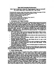
This shows the familiar dataflow network editor where the application is composed. The two panels on the left are the module sets available on two Grid resources – one the desktop, the other a remote server. Modules executing on the remote resource appear as normal in the dataflow network, with full user interface control, and are labelled to show the resource on which they are located. The wind direction widget (top left in the network) is used to steer the simulation according to weather predictions, and the simulation output is displayed in the context of the terrain. In this application, it is useful to collocate the data extraction part of the pipeline with the simulation, so that no unnecessary data is transmitted between remote resource and the desktop. The screenshot of Figure 4 shows the building of the network by a visualization programmer. For the end-user scientist this is encapsulated as an application, with significant control settings promoted to the user interface and wiring diagrams hidden. Different user interfaces can be created for different role players in a collaborative session, as discussed in § 4.2, and Figure 5 shows a collaborative session between an environmental scientist and meteorologist. The scientist runs the simulation but shares steering parameters and visualization with the meteorologist.
Figure 5: Collaboration between scientist and meteorologist endusers
Figure 4: Grid-enabled IRIS Explorer
The Grid can help by providing off-the-shelf compute power to allow scientists to simulate the event in faster than real time. A domain expert can run their atmospheric gas dispersion model and examine the results using visualization. However, as well as computational resources, the scientist needs information from a meteorologist about current weather conditions to steer the simulation. Since time is short, rather than co-locating the scientists, they must be able to collaboratively steer the simulation and visualize the results. Since the decision to order an evacuation will be taken by the local authorities, the visualized data need to be presented in an easy-to-digest form. This requires the visualization tools to be flexible enough to allow different visualizations of the same data to occur, while still remaining under collaborative control. A screenshot of the user’ s desktop for the Grid-enabled IRIS Explorer application is shon in Figure 4.
The dataflow network of Figure 4 was created directly using the IRIS Explorer network editor. Alternatively we can create the dataflow network using the SVG editor described in § 4.3 – as indeed we demonstrate in Figure 6. The corresponding skML document can then be read into IRIS Explorer using the skML interpreter module, to generate the dataflow network of Figure 4. The advantage of this approach is that we have a description of the dataflow network that created the visualization, in a form that is independent of any particular visualization system – important when we wish to consider the issue of provenance. It is important to note that this is only a proof-of-concept demonstrator. The simulation is simplistic, and the terrain equally so. But it is representative of a class of applications where Gridenabled visualization is important, namely, environmental modelling in which maximum compute power is needed to deal with a crisis scenario – and visual analysis by a group of interested parties is vital to decision making. Flood control and forest fire control are two similar applications.
allowing e-scientists to locate running simulations, and connect to them from a front-end application). •
Exploit existing visualization systems: we take the view that we want to re-use existing visualization systems, which are now quite mature, but do not want to prescribe any particular system.
•
Well specified protocol for communication between front and back ends: we have defined a simple XML application for this communication.
•
Distinguish fixed and variable parameters: some parameters must remain fixed for the duration of a simulation to maintain integrity of the physics, or the numerical approximation (some of these are output by the simulation itself, such as current integration step-size and are of interest, but in a ‘read-only’ sense); others are truly steerable (such as frequency of output).
•
Manage different rates of producer-consumer: the simulation produces data that the front-end interface consumes, but the rates will be different – therefore we need to have a strategy that accommodates this. For example, if the simulation generates data sets faster than the visualization system can visualize them then we need to either: skip intermediate data; or cache data between the simulation and the visualization system; or request the simulation slows down while the visualization system is attached.
•
Support collaboration: we want to allow many simultaneous front-end processes to be able to connect, and we want the output to them to be synchronised.
Figure 6: SVG editor being used to create a skML version of the pollution dataflow network
6
DE-COUPLING SIMULATION AND VISUALIZATION
6.1 The gViz Library While skML allows us to describe the visualization process in a generic way, it is realised at the physical layer through visualization environments such as IRIS Explorer, AVS, and VTK. These systems are designed to be self contained: in the case of visualization environments, the visualization process is performed by connecting together a set of system specific modules (some of which may be user-created); in other cases the provided visualization functions are compiled together and executed as a single process. In the demonstrator described in §5.3, the modules are able to run on one or more remote Grid resources, but they are all still contained within the one system. The simulation has been coded as a module within the IRIS Explorer framework and is constrained by the limitations thereof. All these systems implement the typical visualization scenario of reading pre-computed data from files on a disk. Many offer the possibility for user extensions to include extra functionality such as numerical simulations. What is not provided is the ability to easily attach these systems to instruments, numerical simulations or other processes already running at other locations on the Grid. This additional functionality would allow users to interact with the process of dynamic data generation while being guided from the visual feedback provided by the visualization process.
We have completed a first implementation of this design as the gViz library. It handles external communications in a way that keeps interruption of the simulation to a minimum. It provides threads to receive changes to steerable parameters and holds them in a queue until requested by the simulation. It also provides threads to serve current parameter values to connected clients and threads to serve computed data.
This has motivated our work to define a library, primarily for computational steering, to allow connection between external components and a front-end visualization system. The library is in two parts: one part provides an API that the e-scientist can use to instrument their simulation code; the other part provides an API that allows matching capability to be integrated into the front-end visualization system. Our design aims include: •
Lack of intrusion: we want to impact as little as possible on the simulation, so that integrating current simulation codes with the library is as easy as possible.
•
Minimise performance loss: we want to maximise the time the simulation spends using the processor for computation by allowing the library to handle external interactions.
•
Breadth of scope: we want to support the steering of both short and long-running simulations (support for long-running implies an ability to connect and disconnect).
•
Exploit service-oriented concepts: we want to be able to view computational steering from a web services angle (thus we aim to see simulations registering with a directory service, depositing information about how to connect –
Figure 7: Using gViz to steer and visualize data from a simulation running on the grid
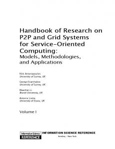
A second component of the library provides API routines for clients to use to create connections to the simulation. These connections are then used to send/receive parameter values in an XML format, or to receive data. This then allows us to view our visualization pipeline in a slightly different light. Rather than having the simulation in the pipeline, we now have modules that represent the control of the simulation and access to the simulation data, but the simulation itself is a separate external process (as shown in figure 7) Communication between simulation and client codes can be handled in a number of ways. The simulation writer determines
this by the method they choose when initialising the library. The simplest method for use within secure environments is to use standard Unix sockets. Alternatively, a web services interface is provided using the gSOAP library [6]. Where access is to be limited to specific users in potentially open environments, then an interface based on Globus sockets is provided. This allows the simulation writer to provide a list of authorised users and hence create limited secure access. Again a web services interface is provided with the gSOAP library but this time using the GSI plugin to provide authentication. Beyond this, encryption can be enabled to allow secure transmission of data. In addition to the gViz library, there are two associated tools: gVizDS and gVizProxy. Since the system is designed to allow user interface applications such as visualization systems to connect to already running processes like numerical simulations, there needs to be a way to locate these processes. When simulations are started they register themselves with a directory service, gVizDS, which holds their connection details. On exit they un-register. This allows visualization systems built using the client component of the library to find the running simulations by contacting one or more gVizDS servers. Once the location of the required simulation is known, the visualization system can contact it directly. gVizDS functionality is provided as a set of web services accessed using SOAP. Many Grid compute resources are comprised of clusters, and typically the internal nodes of clusters are configured as private networks. This makes it difficult for external processes to communicate with processes running on internal nodes since their IP addresses are valid only within the cluster. To form a “bridge” between internal and external processes we use gVizProxy. It is designed to run on a node in the cluster that can see both the external network and the internal nodes, and it registers itself with a copy of gVizDS running on the same node. When visualization applications contact gVizDS to find running simulations, the contact details for gVizProxy are returned, along with those for simulations running on that cluster. The visualization application can then connect to gVizProxy as though it were connecting to the actual simulation, and gVizProxy passes data in and out of the cluster between the simulation and the visualization system. Additionally, if the simulation is using Globus to manage authenticated access, then this can be delegated to gVizProxy. 6.2 Pollution Demonstrator with the gViz Library The demonstrator described in §5.3 uses our extensions to place modules on various Grid resources, selectively sending data/geometry/images back to the desktop. The simulation that is being steered is implemented as one of those modules and is placed on the Grid under the control of the visualization system. Exiting the visualization system terminates the simulation process. In this section, we describe an enhanced version of the pollution demonstrator, in which we use the gViz library to connect the simulation to IRIS Explorer as front-end visualization system. This enables us to launch the simulation code from the desktop, attach to it using control modules in the visualization system for steering and visualization, and then detach at any time leaving the simulation free to continue. At a later time we can restart the visualization system and re-connect to the simulation to monitor its progress. We again exploit the work of § 5 in distributing IRIS Explorer modules: in this version of the demonstrator the modules that connect to the simulation’ s data service can be placed on the same machine/cluster as the simulation. As before this allows us
to filter the data before transmission across the network. We also have modules that connect to the parameter steering/viewing services of the simulation so we can monitor its state and provide new steering parameters if required. The architecture is shown schematically in Figure 8: we see the steering running on the desktop and linked through the gViz library to the simulation running on the remote Grid resource; the visualization pipeline, while designed on the desktop, executes entirely remotely as shown, the data being read from the simulation using the gViz library. The rendered image is then transmitted back to the desktop for display. Thus we demonstrate both the gViz library of § 6.1, and the Grid-enabled IRIS Explorer of § 5.
Figure 8: Connecting simulations and visualization components on the grid
Simulations that are already running are located through gVizDS, the directory service. Simulations connect to gVizDS through a web services interface, at startup, and then contact it again to be removed on exit. A module has been written for IRIS Explorer and is used by the demonstrator to locate already running codes. By using the COVISA collaborative working facilities of IRIS Explorer, we allow teams of scientists to jointly work with the visualization interface. The gViz library has been designed to be independent of any particular visualization system and although IRIS Explorer has mainly been used as the front-end visualization system, we have also used SCIRun, Matlab and VTK. 6.3 Lubrication Simulation with the gViz Library One application at the University of Leeds that has been using this work has been numerical modelling of lubrication. In ongoing work with Shell Global Solutions state-of-the-art software for simulations of elastohydrodynamic lubrication (EHL) has been developed. This particularly challenging problem from mechanical engineering occurs, for example, in journal bearings and gears where, at the centre of the contact, the load exerted over a very small area causes extremely high pressures resulting in elastic deformation of the components and significant changes in the lubricant properties in this area. One of the main research areas in EHL is the modelling of real surface roughness. In these cases, the microscale roughness patterns on the components are simulated rolling through the contact. To accurately resolve these features it is necessary to use very high mesh resolutions and hence parallel computing techniques. It has been shown how such techniques can be combined with a PSE (Problem Solving Environment) for realtime visualization of these parallel simulations [8]. This has now been extended into fully independent Grid applications through
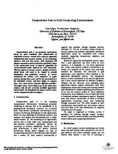
the use of the gViz library. This allows the launching of the parallel EHL code as well as interaction with the fluid, physical and numerical parameters of the simulation while it executes. It also allows changes to the roughness patterns to be made, and automatically receives data for visualization as it is produced. A screenshot illustrating the ECLIPSE PSE is shown in Figure 9.
Figure 9: ECLIPSE PSE
7 CONCLUSIONS AND FUTURE WORK This paper has explored how dataflow visualization can evolve into the era of Grid computing. We have split the traditional reference model into layers of increasing specification in terms of software and hardware resources, with an XML language representation for dataflow at the different levels. This has driven a Grid-enabled extension of an existing dataflow visualization system, IRIS Explorer. For challenging computational steering applications, we have developed a library allowing connection of remote simulations with front-end visualization systems. This allows a scientist to monitor a range of running simulations, with the desktop acting as a control deck from which operations are managed. We see our work as a contribution to evolving concepts and software for visualization in Grid environments. It has wide applicability. The skML work is based on standard Web technologies, and offers a system-independent description of a dataflow network. The gViz library will be available as open source, and its generality has been demonstrated through use with IRIS Explorer, Matlab and VTK. Our research is now turning to the transition between the layers in the reference model. Can we allow the user to work at the conceptual layer, designing the visualization intent through a Grid portal, and have the allocation of software and hardware resources determined by a brokering agent? ACKNOWLEDGEMENTS This work was carried out within the gViz project funded under the UK e-Science Core Programme and we gratefully acknowledge their support. The technical development work reported here was principally carried out by Jason Wood (University of Leeds) and Musbah Sagar (Oxford Brookes University), under guidance of Ken Brodlie and David Duce respectively. Chris Goodyer and Mark Walkley (University of Leeds) created the simulation software. Ying Li and James Handley (University of Leeds) created the VTK and Matlab interfaces. Other key members of the project team include Mike Giles and David Gavaghan (University of Oxford); Steve Hague (NAG Ltd); Mike Rudyard (Streamline Computing Ltd); and
Brian Collins, Alan Knox and John Illingworth (IBM UK Ltd). We are also grateful to Arun Holden (University of Leeds) and Richard Clayton (University of Sheffield). REFERENCES [1]
Brodlie, K.W., Duce, D.A., Gallop, J.R., Walton, J.P.R.B. and Wood, J.D. 2004. Distributed and Collaborative Visualization, Computer Graphics Forum 23, 2, 223-251.
[2]
Cactus 2004. http://www.cactuscode.org.
[3]
Charters, S., Holliman, N.S. and Munro, M. 2003. Visualization in e-Demand: A Grid Service Architecture for Stereoscopic Visualization, Proceedings of UK e-Science Second All Hands Meeting.
[4]
Chin, J., Harting, J., Jha, S., Coveney, P.V., Porter, A.R. and Pickles, S.M. 2003. Steering in Computational Science: Mesoscale Modelling and Simulation, Contemporary Physics 44, 417-434.
[5]
CC/PP 2004. http://www.w3.org/TR/2004/REC-CCPP-struct-vocab-20040115/
[6]
van Engelen, R., Gupta, G. and Pant, S. 2003. Developing Web Services for C and C++, IEEE Internet Computing 7, 3, 53-61.
[7]
GLUE 2004. http://www.globus.org/mds/glueschemalink.html
[8]
Goodyer, C.E., Wood, J.D. and Berzins, M. 2002. A Parallel Grid based PSE for EHL Problems. In: Applied Parallel Computing Advanced Scientific Computing 6th International Conference, PARA 2002, Fagerholm, J., Haataja, J., Järvinen J., Lyly, M., Råback, P. and Savolainen, V., Eds, Springer Verlag, 521-530.
[9]
Haber, R.B. and McNabb, D.A. 1990. Visualization Idioms: A Conceptual Model for Scientific Visualization Systems. In: Visualization In Scientific Computing, Shriver, B., Neilson, G.M., and Rosenblum, L.J., Eds., IEEE Computer Society Press, 74-93.
[10] McCormick, B.H., DeFanti, T.A. and Brown, M.D. 1987. Visualization in Scientific Computing, Computer Graphics 21, 6. [11] Marshall, R., Kempf, J., Dyer, S. and Yen, C. 1990. Visualization Methods and Simulation Steering for a 3D Turbulence Model for Lake Erie, ACM SIGGRAPH Computer Graphics, 24, 2, 89-97. [12] RDF 2004. http://www.w3.org/RDF/ [13] RSL 2004. The Globus Resource Specification Language (RSL). http://www.globus.org/gram/rsl_spec1.html [14] Shalf, J. and Bethel, E.W. 2003. The Grid and Future Visualization System Architectures, IEEE Computer Graphics and Applications 23, 2, 6-9. [15] Suzuki, Y., Sai, K., Matsumoto, N. and Hazama, O. 2003. Visualization Systems on the Information-Technology-Based Laboratory, IEEE Computer Graphics and Applications 23, 2,32-39. [16] Upson, C., Faulhaber, T., Kamins, D., Schlegel, D., Laidlaw, D., Vroom, J., Gurwitz, R. and van Dam, A. 1989. The Application Visualization System: a Computational Environment for Scientific Visualization, IEEE Computer Graphics and Applications 9, 4, 3042. [17] Walton, J.P.R.B. 2004. NAG' s IRIS Explorer. In: Visualization Handbook, Johnson, C.R. and Hansen, C.D., Eds., Academic Press (in press). Available at http://www.nag.co.uk/doc/TechRep/Pdf/tr2_03.pdf. [18] Wood, J.D., Wright, H., and Brodlie, K.W. 1997. Collaborative Visualization. In: Proceedings of IEEE Visualization ' 97, Yagel, R., and Hagen, H., Eds., 253-259. [19] XGMML 2004. http://www.cs.rpi.edu/~puninj/XGMML/