Hans Hagen†. Heinz Krüger‡. Martin Menzel§. Alyn Rockwood¶. Figure 1: A transformer. Abstract. We present an algorithm for the visualization of vector field.
Visualization of Higher Order Singularities in Vector Fields Gerik Scheuermann∗
Hans Hagen†
Heinz Kr¨uger‡
Figure 1: A transformer
We present an algorithm for the visualization of vector field topology based on Clifford algebra. It is the first method allowing the detection of higher order singularities. This is accomplished by first analysing the possible critical points and then choosing a suitable polynomial approximation because conventional methods based on piecewise linear or bilinear approximation do not allow higher order critical points and destroy the topology in such cases. The algorithm is still very fast because of using linear approximation outside the areas with several critical points.
1
Introduction
Since Helman and Hesselink [3, 4] introduced the method of visualizing the topology of vector fields there has been a big interest in this kind of vector field visualization. But all methods so far begin with linear or bilinear interpolation of the grid data and start the analysis of the topology from there. This is a fast algorithm and one gets good results as long as the critical points are well separated and of simple type. But this is often not the case and then the linear or bilinear interpolation of the grid cells reduces artificially the possible topological structure as we will see, especially it makes the existence of critical points of index higher than 1 or lower than -1 impossible. This drawback let us look for different ways to analyse the topology without losing the advantage of the high speed in the conventional methods because of the big datasets occuring from all kind of vector field simulations. The starting point is to look for areas where higher order critical points are possible and then use a polynomial approximation of sufficient degree in that area to allow critical points of maximum resp. minimum order. Outside these ∗ Department
of Computer Science, University of Kaiserslautern of Computer Science, University of Kaiserslautern ‡ Department of Physics, University of Kaiserslautern § Department of Physics, University of Kaiserslautern ¶ Department of Computer Science, Arizona State University † Department
Alyn Rockwood¶
areas we still use the linearization of the field. This is normally the whole field except for some small but very important areas so that the algorithm is not loosing its capability of analysing big datasets. Typical applications are the magnetic fields inside coils or transformers like the one in figure 1. Several windings construct a higher order singularity. The eddy motions in turbulent flows are also a source for higher order critical points. More examples can be found in all kind of fields with symmetry conditions preventing the critical points from splitting into several simple points. We do not know about papers dealing with the visualization of higher order singularities in vector fields, so this is the first article dealing with this problem. Clifford algebra is used in [7] to analyse the topology of planar polynomial vector fields which also gives the mathematical background in more depth than this paper. Here we show how this results can be used for the visualization of vector fields.
2 Abstract
Martin Menzel§
Higher order singularities
Since the very start of the visualization of vector field topology there has been said much about critical points in a vector field so a short remark should be enough for the simple case. A critical point of a real 2D-vector field v : R2 → R2
(1)
(x, y) 7→ (v1 , v2 )
2
is a point P ∈ R where the vector field vanishes. If the derivative of v at P DP v : R 2 → R 2 (2)
�
x y
�
7→
�
∂v1 ∂x ∂v2 ∂x
∂v1 ∂y ∂v2 ∂y
��
x y
�
has full rank, one gets the simple critical points with their classification by the eigenvalues of DP v as in [6, p.96] and the well known patterns of figure 2. If DP v has one or two zero eigenvalues, more complex topological patterns around P can appear. The most important invariant for the behavior in the neighborhood of the critical point is the Poincar´e-Hopf index or winding number indp v = indγ v =
1 2π
Z
v1 dv2 − v2 dv1 v12 + v22
(3)
γ
where γ : S 1 → R2 is a closed curve making one turn in counterclockwise sense around P and containing no other zeros of the field [1, p. 320]. In the figure 3 one can see the classical computation by the number of turns of the field around the critical point. Some typical examples for higher order critical points are given in figure 4. Our main goal is now to get a visualization with critical points having the right index. This means that we need simple descriptions of critical points with a given index. An easy way is given by complex analysis as is shown for example in [2, p. 53]. Let
γ
Figure 3: Index computation at a star. The field makes one counterclockwise turn along γ, so the star has index +1.
index +2
index +3
index -2
index -3
Figure 4: Higher order critical points
repelling spiral
saddle
repelling node
E(z)=z2
E(z)=z
Figure 5: Complex description of critical points with positive index attracting spiral
circle
attracting node
Figure 2: Simple critical points
z 7→ z˜k Again the field in real coordinates is
z = x + iy be a complex variable for identifying R2 and C and look at the vector field in the complex plane given by E:C→C
(4)
In real coordinates one gets the field
(x, y) 7→ (Re(z k ), Im(z k ))
(7)
(x, y) 7→ (Re(˜ z k ), Im(˜ z k ))
z 7→ z k
v : R2 → R2
v : R2 → R2
(5)
For k = 1, 2 this produces the phaseportraits in figure 5 and it is quite easy to see that the vector field E has always only one zero at the origin with index −k. For a negative index one uses the complex conjugate z˜ = x − iy and defines E:C→C (6)
with the structure as shown in figure 6 for k = 1, 2. In case (4) with k > 1 we find 2k − 2 curves going to infinity or coming from there and all other curves start at the critical point and converge again at it, producing 2k − 2 elliptic sectors. An exact analysis of the integration curves around the zeros of the field (6) shows that only 2k + 2 curves converge to the critical point. They separate the neighborhood into 2k + 2 hyperbolic sectors. It may be emphasized that elliptic sectors are impossible in the linear case and that z 2 gives the well-known dipole pattern. In section 5 we show what happens to such a field if one uses standard linear approximations.
E(z)=z~
E(z)=z~2 ¯ ¯ Figure 7: E(r) = ze1 and E(r) = z˜e1
Figure 6: Complex description of critical points with negative index
3
Clifford vectorfields
Clifford algebra extends the classical description of an euclidean nspace as a real n-dimensional vector space with scalar product to a real algebra. It simply gives a way to multiply vectors in arbitrary dimensions and get a geometric interpretation of the result [5]. In our 2D-case it also gives a way to describe the relation between real and complex numbers in a nice way. For the euclidean plane we get a 4-dimensional R-algebra G2 with the basis {1, e1 , e2 , i = e1 e2 } as a real vector space. The multiplication is defined as associative, bilinear and by the equations 1ej ej ej i = e 1 e2
= = =
ej j = 1, 2 1 j = 1, 2 −e2 e1
(8) (9) (10)
The usual vectors (x, y) ∈ R2 are identified with xe1 + ye2 ∈ E 2 ⊂ G2
(11)
and the complex numbers a + bi ∈ C with For a real vector field
a1 + bi ∈ G2
(12)
v : R2 → R2
(13)
¯ Figure 8: E(r) = i˜ z e1 In general one can easily show that for ¯ E(r) = (az + b˜ z + c)e1
(16)
with a, b, c ∈ C one gets all linear fields. For higher order critical points we meet our examples from section 2 again, but the roles of z and z˜ have changed. Examples 2 9
¯ (4) E(r) = z 2 e1 gives the monkey saddle in figure
¯ (5) E(r) = z˜2 ze1 gives a dipole as in figure 9
(x, y) 7→ (v1 , v2 )
one sets the Clifford vector field
¯ : E2 → E2 E
(14)
r = xe1 + ye2 7→ v1 e1 + v2 e2
This is trivial but with z = x + iy, z˜ = x − iy one can interpret this as ¯ E(r) = E(z, z˜)e1 (15) where E : C 2 → C is a complex function of two complex variables. Some examples may illustrate now the results of this mathematical transformation. Examples 1
¯ (1) E(r) = ze1 gives the saddle in figure 7
¯ (2) E(r) = z˜e1 gives the star in figure 7 ¯ (3) E(r) = i˜ z e1 gives the circle in figure 8
¯ ¯ Figure 9: E(r) = z 2 e1 and E(r) = z˜2 e1 A generalization of this examples is given by the following theorem. ¯ : E 2 → E 2 ⊂ G2 be a Clifford vector field Theorem 1 Let E with ¯ E(r) =a
n1 Y j=1
n1 +n2
(z − zj )kj
Y
j=n1 +1
(˜ z − z˜j )lj e1
(17)
and a, z1 , . . . , zn ∈ C, n = n1 + n2 . ¯ zeros at z1 , . . . , zn and nowhere else and the index of Then has E ¯ at zj is lj − kj . E
-1
A proof will appear in [7].
-1
4
Detection of higher order singularities
The conventional method for analysing the vector field topology starts with a piecewise linear or bilinear approximation and analyses the topology of the approximated vector field. The problem is that one never gets critical points with an index bigger than 1 or smaller than -1. Consequently we use a different way. If the selection of the approximation determines the possible critical points one should first look at the data, analyse the possible indices and then approximate in a way allowing every possible index at the critical points inside an area. The index integral (3) has the nice property to be additive on closed curves in the following sense : If one has a boundary curve C of an area and divides that area into two parts with boundaries C1 , C2 like figure 10, one has : indC v = indC1 v + indC2 v
Figure 12: Indices around a monkey saddle
with a, b, c ∈ C for our visualization. The last section showed that this allows two saddles or a monkey saddle, so we can get the right index. In the case of a positive index as in figure 13 we use an approximation of the type ¯ E(r) = b(˜ z−a ˜1 )(˜ z−a ˜2 )e1
(20)
to allow higher order critical points in this situation.
(18)
+1 C C2
+1
C1
Figure 13: Indices around a dipole
Figure 10: A curve splitted into two If we take now an arbitrary triangulation or grid, we can compute the index of every curve along the grid edges by computing the index of each cell and adding the indices of the cells inside our curve as in figure 11.
5
+1 -1
There is obviously no problem with an arbitrary index in the light of section 3. After this step we check if the distance between some of the ai is below a wished quality limit and if so we assume a higher order singularity by setting these ai to their gravity point. In this way we are able to detect higher order singularities as we will show in the examples in the next section.
-1
-1
Figure 11: Summing the index in a region We now assume for a moment that the vector field is linear along the edges. This allows to compute all indices of the triangles and by the consideration above along each closed sequence of grid edges. If we now have a higher order critical point P , we make a mistake in the triangle or cell containing P but it is not difficult to see that we are not making a mistake if we go around a big enough region containing the point. For index -2 we can get a situation like figure 12. If we would use linear interpolation in each triangle we would get two saddles, but in reality there is only one critical point. In a situation like figure 12 we put all the triangles there in a region and use an approximation of the type ¯ E(r) = b(z − a1 )(z − a2 )e1
(19)
Examples
In the following examples we analyse vectorfields with known topology by our algorithm and compare it with the conventional piecewise linear method. Our first example is just a monkey saddle. Figure 14 shows the linear approximation of the field around a monkey saddle on a 20x20 quadratic grid and a zoom into the interesting part. Instead of one critical point of higher order one gets four critical points in that area. The results of our algorithm can be seen in figure 15. After these easy example we are now going to look at two steps of two saddles approaching each other and merging into a monkey saddle together with four index 1 singularities with fixed locations. This kind of example was computed by the methods developed in [7] based on Clifford algebra by extending the technique given in section 3. We used again a quadratic 20x20 grid with [−1, 1] × [−1, 1] as bounding box. The results can be seen in figure 16 to 19. The distance d between the two saddles was 0.0250 and 0.0000. The missing fourth separatrix of the right saddle in figure 18 comes from the fact that the saddle is close to a triangle where the main direction of the flow goes down, so that the algorithm puts this backward computed separatrix over the one coming from the source in the upper right corner.
6
Acknowledgment
This work was partly made possible by financial support by the Deutscher Akademischer Auslandsdienst (DAAD). The first author got a ”DAAD-Doktorandenstipendium aus Mitteln des zweiten Hochschulsonderprogramms” for his stay at the Arizona State University from Oct.96 to Jan.97. We like to thank for this support which helped to continue our cooperation.
References [1]
V I. Arnold. Gew¨ohnliche Differentialgleichungen. Berlin, Deutscher Verlag der Wissenschaften, 1991.
[2]
J. Guckenheimer, P. Holmes. Nonlinear Oscillations, Dynamical Systems and Bifurcation of Vector Fields. Springer, New York, 1983.
[3]
J. L. Helman, L. Hesselink. Automated Analysis of Fluid Flow Topology. 3D Visualization and Display Technologies (Proc. SPIE) Vol. 1083, SPIE, Washington Jan. 1989, pp. 825-855.
[4]
J. L. Helman, L. Hesselink. Representation and Display of Vector Field Topology in Fluid Flow Data Sets. Computer, Vol. 22, No. 8, Aug. 1989, pp. 27-36.
[5]
D. Hestenes. New foundations for classical mechanics. Kluwer Academic Publishers, Dordrecht, 1986.
[6]
M. W. Hirsch, S. Smale. Differential Equations, Dynamical Systems and Linear Algebra. Academic Press, New York, 1974.
[7]
G. Scheuermann, H. Hagen, H. Kru¨ ger. An interesting class of polynomial vector fields. submitted to Mathematical Methods for Curves and Surfaces II, M. Dæhlen, T. Lyche, L. L. Schumaker (eds.).
Figure 14: Linear approx. around monkey saddle
Figure 15: New approx. around monkey saddle
Figure 16: Linear approx. for d=0.0250
Figure 17: New approx. for d=0.0250
Figure 18: Linear approx. for d=0.0000
Figure 19: New approx. for d=0.0000