fourth order material tensor but despite of painting complex glyphs, no method .... decomposition of the matrix representation of second order tensors, especially.
Tracking Lines in Higher Order Tensor Fields Mario Hlawitschka and Gerik Scheuermann Department of Computer Science University of Leipzig PF 100920 D-04009 Leipzig Germany {hlawitschka|scheuermann} @ informatik.uni-leipzig.de
Abstract. While tensors occur in many areas of science and engineering, little has been done to visualize tensors with order higher than two. Tensors of higher orders can be used for example to describe complex diffusion patterns in magnetic resonance imaging (MRI). Recently, we presented a method for tracking lines in higher order tensor fields that is a generalization of methods known from first order tensor fields (vector fields) and symmetric second order tensor fields. Here, this method is applied to magnetic resonance imaging where tensor fields are used to describe diffusion patterns for example of hydrogen in the human brain. These patterns align to the internal structure and can be used to analyze interconnections between different areas of the brain, the so called tractography problem. The advantage of using higher order tensor lines is the ability to detect crossings locally, which is not possible in second order tensor fields. In this paper, the theoretical details will be extended and tangible results will be given on MRI data sets.
1
Introduction
Tensors are mathematical objects that are used in physics and engineering for measuring natural quantities or for describing derived quantities such as the vector derivative which is a second order tensor. While second order tensors, especially symmetric second order tensors are well studied and many visualization techniques exist, little has been done to visualize tensors of order higher than two. Higher order tensor occur for example in mechanical engineering as the fourth order material tensor but despite of painting complex glyphs, no method exists for analyzing the structure of higher order tensor fields. Magnetic resonance tomography (MRT) is an imaging technique used in medicine that is more sensitive to tissue structures than computer tomography (CT). Diffusion weighted MRT is a variant where diffusion of hydrogen bound in molecules is measured along gradient directions of an applied magnetic field. As the magnetic field gradient can be changed, the diffusion can be sampled using a three dimensional sampling pattern. If six different directions on a sphere g (i) are acquired leading to six signals s(i) , i ∈ {1 . . . 6} measured in addition to a
base image s(0) , a second order diffusion tensor can be reconstructed by solving the system of six equations (i)
s(i) = s(0) e−bTjk gj
(i)
gk
(1)
describing a symmetric second order tensor1 Tjk = Tkj . Here s(i) is the signal intensity in presence of a magnetic field gradient and s(0) is the baseline image which is the signal intensity in absence of diffusion-sensitizing field gradients to which the remaining measurements are related. The parameter b is called bfactor or diffusion weighting factor which will be assumed to be a constant here. The influence of the b-value to the measurement has been studied for example by Frank [1] and Jones [2]. Usually, more gradient directions are used to smooth the data and equation 1 is solved using least squares fitting. In addition to this approach, other techniques have been introduced to handle the additional information gained by sampling using more than six points, among these are q-Space imaging, higher angular resolution diffusion (tensor) imaging HARD(T)I and q-Ball imaging. While q-Space imaging [?] is difficult to measure and is prone to artefacts [3], q-Ball imaging needs a high number of gradient directions (about 120 to 300) [3]. HARDI is a technique using higher order tensors to represent diffusion patterns using higher angular resolution than second order diffusion tensor imaging while only a reasonable small amount of gradient directions is needed. The number of gradient directions is important because of its linear dependence on the measuring time. In clinical environments only ten to twenty minutes of scanning time are available resulting in six to thirty gradient directions using two or three images for averaging. Concerning visualization, the ellipsoidal glyph is a rather simple but the best known visualization technique. It is an ellipsoid spanned by the scaled eigenvectors of the symmetric, positive definite second order tensor and may be interpreted as an isosurface of the density function of particles placed in a fluid after a certain diffusion time. In addition many other glyphs exist like the superquadric glyph presented by Kindlmann [4]. It presents a better technique providing a direction independent interpretation by reducing errors of introduced by visual artifacts. Unfortunately, the physical interpretation partly vanishes. Tensor lines are a well known and widely used method for visualizing symmetric second order tensor fields which are applied in many different settings like mechanical engineering [5, 6] and medical imaging [7]. In MRT of the human brain, neural fibers hinder diffusion perpendicular to their course. Therefore tensor lines approximate the neural fiber structures found in the white matter of the brain. While second order tensors can represent only a single direction (the direction of the major eigenvector discarding its orientation), higher order functions are able to represent a higher angular resolution and thus a higher amount of directions inside the same volume element. This makes it possible to extract 1
We use Einstein’s summing convention in all equations where variables are summed up over same indices on one side of the equation. Free indices or indices on different sides of the equation lead to a system of equations.
a higher amount of information from the scanned data compared to simple second order tensor approaches. Usually crossings are detected by looking at the neighboring voxels which reduces the absolute resolution of the data. As current diffusion tensor images still have a relatively low resolution (usually larger than 1 × 1 × 1mm3 compared to the fiber structures which are at a resolution of micrometers in diameter) and many fiber tracts span only across two or three voxels, it is important to work with the highest resolution of data available. This implies that analysis of data at voxel resolution or beyond is crucial for analyzing MRT data.
2
Higher Order Tensors
A tensor of order (rank)2 r and dimension d is a multilinear form mapping r d-dimensional vectors to a scalar: r
T : (Rd ) → R � � (r) (1) v(1) , . . . , v(r) → Ti1 ...ir · vi1 · · · vir .
(2) (3)
When using the same normalized direction vector g (we call it gradient vector as used in the MRT nomenclature) a tensor can be interpreted as a scalar function defined on the sphere (i) (i) (4) fT (g) = Tj1 ...jr · gj1 · · · gjr There is an analogy between symmetric even order tensors and the symmetric spherical harmonics approach presented by Frank [8] which has been pointed ¨ out by Ozerslan et al. [9]. This can be used as an alternative to the tensor representation. A discussion of the use of spherical harmonics in detail can also be found in Hlawitschka et al. [10]. Here we only want to emphasize the similarity of the spherical harmonic transform to the Fourier transform. Thus, higher order spherical harmonic basis functions contain higher frequency components. As spherical harmonics and the tensor functions fT of same order r describe the same function space, the frequency information is contained in the tensors, too. We compute a higher order tensor using the raw information s(0) and s(n) and map it to a tensor T of order r using s(n) = s(0) e−bTi1 ...ir ·gi1 ···gir
(5)
To display this information, we use a generalization of Reynold’s stress glyph that is defined by the surface S = {p ∈ R3 : pj = Ti1 ...ir · vi1 · · · vir · vj 2
∧
v ∈ S 2 }.
(6)
We are ignoring the difference between contravariant and covariant indices here and use a fixed orthonormal coordinate system for the sake of readability. Therefore all tensor indices are lower indices and vector indices should be interpreted as upper indices to preserve mathematical correctness but are written as lower indices to simplify notation and to allow upper indices to be reused differently where needed.
The usual color map for medical imaging indicating the direction of the largest expansion can be applied to this, too, as shown in Fig. 1. Fading out the color by anisotropy values is difficult for higher order tensors because anisotropy measures of higher order tensors can not be compared to those of second order tensors. This is due to the fact that higher order components are independent of lower order components. Color mapping on the surface function can be applied to strengthen the shape of the glyph. In addition, arrows can be drawn to improve visibility of local maxima as shown in Figures 2–5 and 8.
Fig. 1. A comparison of different tensor glyphs in the area marked by the red box including parts of the forceps minor and the pyramidal tract. Middle: Box glyphs aligned to the eigenvectors (left) and Superquadric tensor glyphs (right). Bottom: second order Reynold’s glyph (left) and its fourth order modification (right).
Fig. 2. First order tensor are defined by the scalar product of the direction vector and the vector sampling the surface. It is obvious that lines can be drawn and that they correspond to streamlines. (The scaling of the sampling vector has been normalized for this drawing, blue values are negative.)
Fig. 3. Second order tensor lines in general have one major eigendirection. They also are a subset of fourth order tensors.
Fig. 4. Symmetric, fourth order tensors may have more directions and have special degenerated cases like the one in the middle where a single major direction still exists.
Fig. 5. Our approach of tracking lines is also applicable to mixed order tensors (here zeroth and third order), but this is not investigated any further due to the lack of application.
3
Higher Order Tensor Lines
Despite of the fact that glyphs give a good impression of the properties of a tensor defined at a certain position, no information is shown about its neighborhood. Therefore stream lines and tensor lines have been introduced to depict the information present in a certain neighborhood around a point of interest or – when using randomly seeded lines or lines seeded by complex algorithms determining good seed points – global information about the behavior of the vector or tensor field. Therefore, tensor lines have been used in many fields of visualization. Even though tracking of second order tensor lines reveals a reasonable visualization for medical images on the first view, it does not handle crossings of fibers at all due to its nature and underlying model of gaussian diffusion. Thus, the interconnections between the inner part of the corpus callosum and the outer areas of the corpus callosum are not handled correctly because they seem to be divided by the pyramidal tract. For a detailed description about the commissural fibers (neofibrae commissurales) from a neurological/topical point of view refer to Duus [11]. In second order tensor fields these techniques are based on the eigenvector decomposition of the matrix representation of second order tensors, especially symmetric, positive definite tensors which have three positive eigenvalues and three orthogonal eigenvectors. As there is no such decomposition for higher order tensors [12], we introduce a technique leading to the same results for stream lines and tensor lines that is applicable to higher order tensor fields, too.
Fig. 6. A second order Reynold’s glyph with maxima and minima indicated by red and blue arrows resp. and its eigenvector decomposition (thin green lines).
A non degenerated symmetric second order tensor as shown in Fig. 6 has two distinct maxima, two minima and two saddle points which correspond to its eigenvector directions. We use this property to define a major tensor line as a line following these maxima. Let Σ be the set of tensors of arbitrary order r and let T : R3 ⊇ U → Σ p → T (p)
(7) (8)
be a C 2 continuous tensor field. In the following, we study the corresponding function fT (p) at each position, i.e. fT (p) : S 2 → R (θ, φ) → fT (p) (θ, φ)
(9) (10)
so we have a function on the sphere at every position. Definition 1. We call a position p ∈ U degenerated if there is a position (θ, φ) ∈ S 2 where (11) ∇S 2 fT (p) (θ, φ) = 0 and det |∇2S 2 fT (p) (θ, φ)| = 0.
(12)
(The name is well chosen because some tensor lines are not uniquely defined at these positions in accordance to the usual notion of degenerate points introduced by Delmarcelle and Hesselink [13]. Fig. 8 gives a visual impression of some of those tensor glyphs.) Usually, testing higher derivatives would lead to a more restrictive definition of degenerated points. There are special instable cases in which study of higher order derivatives would reveal, that what we call degenerated is not degenerated. For simplicity, we ignore these very rare cases in the following sections. At a regular point (i.e. a point that is not degenerated) q ∈ U , we have a finite number M of isolated maxima m1 , . . . , mM = (θ1 , φ1 ), . . . , (θM , φM ) of fT (q). Using the implicit function theorem, we obtain neighborhoods U1 , . . . , UM ⊂ U and unique C 1 continuous functions wm : Nm → S 2 p → wm (p) = (θm (p), φm (p))
(13) (14)
that parametrize the maxima (θm (p), φm (p)) in the neighborhood Nm , i.e. we can extract M C 1 -continuous vector fields around p as shown in Fig. 7. Using these vector fields on Nm we define major arbitrary order tensor lines. Definition 2. A unique (major) tensor line in the tensor field T through the point q following a maximum m is a curve xm : Im → Nm t → xm (t)
(15) (16)
xm (0) = q
(17)
∂xm (t) = wm (xm (t)). ∂t
(18)
with and
Fig. 7. A tensor T at a position p in the data set with two maxima m1 and m2 provides two neighborhoods N1 and N2 around p. On both neighborhoods a C 1 continuous vector field is defined. Because the area contains no critical points, streamlines can be integrated everywhere in the neighborhood. Both sets of lines are combined to areas containing two, one or no streamlines. Usually only lines going through the point p are of interest.
4
Properties of Higher Order Tensor Lines
Similar definitions can be given for minor tensor lines following the minima and medium tensor lines following the directions of saddle points of the functions fT . This provides us with a framework of lines in arbitrary order tensor fields where crossing is a valid behavior of lines following different maxima in overlapping areas. Every parameterized line is uniquely defined by a position and an initial oriented direction. In symmetric tensor fields, two lines having the same direction but different orientation differ in their parameterization only by the relation of their parameters t1 = −t2 . In the following sections, we will deal only with symmetric tensors. As the number of maxima on the function fT is even because of its symmetry, we will speak of one (two, three...) direction when having two (four, six...) maxima of fT . Despite of the fact that our definition of higher order tensor lines is closely related to the definition of second order tensor lines it is independent of the order of the tensor. Thus, this definition can be applied to zeroth, first and second order tensors, too. Obviously, for a zeroth order tensor fT is constant which is also the most important degenerate case in higher order tensor fields i.e. a completely isotropic tensor.
Fig. 8. A fourth order tensor glyph showing two main directions of diffusion (left) and a degenerated fourth order glyph with a single main direction and a “degenerated ring” (right).
4.1
First Order Tensors
First order tensors (vectors) are simply build by the scalar product of the vector direction and the sampling direction v. fT = Ti vi =< T, v >= kT kkvk cos γ,
(19)
thus its maximum in the non degenerated case is in the same direction as the vector direction and our higher order tensor lines correspond to streamlines. A special case about asymmetric functions fT is that there exists a minimum that can be tracked leading to an reverse parameterized line. In the case of first order tensor fields, there is only one minimum which describes backward integration of the streamline. The only degenerated case here is Ti = 0, thus fT = 0. 4.2
Symmetric Second Order Tensors
For symmetric second order tensors, the maximum is in the direction of the largest eigenvector. This can be seen by decomposing T into R−1 DR where R is a rotation of the eigenvector basis of the tensor to the cartesian basis vectors and Dii = λi a diagonal tensor containing the eigenvalues. For a vector e(k) along the k-th eigendirection of T , fT can be written as (k) (k)
fT (e(k) ) = Tij ei ej
(k) (k)
= λ1 ej ej
= λ1 ke(k) k2 .
(20)
For any other direction, the vector v can be projected into the basis of the tensor which can be expressed by the rotation v ˜ = Rv. Let e(k) now be the normalized eigenvectors of the tensor then fT (v) = fT (˜ v1 e(1) + v ˜2 e(2) + v ˜3 e(3) ) (1)
(1)
(2)
(2)
= Tij v ˜1 ei v ˜1 ej + Tk` v ˜2 ek v ˜1 e` + Tmn v ˜3 e(3) ˜1 e(3) m v n = λ1 v ˜12 + λ2 v ˜22 + λ3 v ˜32
(21)
Obviously the maximum of fT for a constant length of v is reached at v ˜1 → max which is achieved by turning the vector v in the direction of the eigenvector of the largest eigenvalue λ1 . This shows that higher order tensor lines are the same lines as second order tensor lines. Due to the fact that the neighborhoods are areas of smooth behavior, their borders have to be degenerated. Even though this seems obvious their calculation and mathematical analysis is still an open topic and will be a subject of further research.
Fig. 9. Slice through a human brain. Top left: Kindlmann’s superquadric glyphs, right: Full brain tracking of second order tensor lines colored by direction. Bottom left: second order tensors displayed by surface glyphs. Bottom right: Fourth order glyphs shown in the same dataset. The red glyphs indicate crossings where the fourth order glyph reveals much more information than the corresponding second order glyph in the same data set. The data set has been provided by Max-Planck-Institute for Human Cognitive and Brain Sciences Leipzig.
5
Application to Real World Data Sets
We applied the method to several measured data sets of healthy volunteers. 36 gradient directions are measured in addition to the base image. The data has been converted to symmetric tensors using equation 4. No additional filtering or smoothing has been applied. The data set consists of a rectilinear grid of size 128 × 128 × 44 with a voxel size of approximately 1.7 × 1.7 × 3.0mm3 . Lines are seeded at every grid point inside the brain or randomly in an region
of interest. We tracked several lines in areas where crossings are assumed in medical literature, e.g. in Duus [11], most important the area close to the corpus callosum. 5.1
Second Order Tensor Lines
Second order tensor lines are used to compare our results to previous results. We seeded a second order tensor line at every position of the grid inside the brain where the fractional anisotropy is larger than 0.2. All lines were stopped when the FA reaches the threshold of 0.15. The resulting lines were filtered by a maximal length of about the diameter of the brain and maximal number of steps to prevent loops and a minimal length of 30mm to remove visual clutter from too short lines. Results of the tracking can be seen in Fig. 9. We further magnified the area where the corpus callosum and the pyramidal tract meet as described by Duus. This area is shown in Fig. 10. Due to limitations of second order tensors tensor lines from the bottom to the top (blue) split the image into two parts. This separatrix cannot be crossed by other lines which can be clearly seen in the figure. 5.2
Higher Order Tensor Lines
The higher order approach has been applied to the same data set. Again, no filtering has been applied. Fourth order tensors are reconstructed as described previously. Random seedpoints have been selected in a region of interest which is approximately the area of the assumed crossing and are marked by different colors than the lines themselves. Due to simplicity, a simple Euler approach with adaptive stepsize control has been used for the integration of lines. The result can be seen in Fig. 11. A comparison to the second order tensor lines that can be seen in Fig. 10 shows that the knowledge of physicians is much better represented by the higher order approach as a crossing of lines can be detected and a smaller amount of lines of the corpus callosum is deflected by the influence of the diffusion pattern of the pyramidal tract and the corona radiata.
6
Conclution and Future Work
The theoretical basis of tracking higher order tensor lines has been presented. Proofs of equality to first order and symmetric second order lines have been indicated. Furthermore, we have shown that higher order tensor lines can be applied to noisy medical data sets acquired using diffusion weighted magnetic resonance imaging with a relatively small amount of gradient directions. There, well known crossings of the pyramidal tract and corpus callosum have been reconstructed that are not visible in second order tensor fields. A comparison to images found in medical literature reveals many similarities, like the crossing structure and their directions that can not be present in second order tensor fields. Further investigations have to be done relating the influence of noise in
Fig. 10. Crossings of the pyramidal tract and the corpus callosum shown using second order tensor lines in a measured data set of a young healthy volunteer. Even though a crossing is expected, second order tensors are not capable of displaying crossing behavior. Data set provided by Max-Planck-Institute for Human Cognitive and Brain Sciences Leipzig.
Fig. 11. Similar view of the same data set as in Fig. 10. Crossings of the pyramidal tract and the corpus callosum painted as tubes. Colored points indicate the random seeding points of the lines. The data set has been provided by the Max-Planck-Institute for Human Cognitive and Brain Sciences Leipzig.
second and higher order tensor fields, describing the reliability of the tracking. Application to other higher order tensor data such as complex fourth order material tensors is still an open topic.
Acknowledgements We thank our cooperation partners from the Max-Planck-Institute for Human Cognitive and Brain Sciences Leipzig especially Marc Tittgemeyer, Alfred Anwander, Thomas Kn¨ osche and Harald M¨oller for providing the data sets, for the fruitful discussions and for answering our questions relating MRT and neuro sciences in general. Further thanks go to Enrico Kaden and Davide Imperati for their useful hints relating the data sets. Finally we thank the FAnToM team for providing the framework for our implementation.
References 1. Frank, L.R.: Anisotorpy in high angular resolution diffusion-weighted MRI. Magnetic Resonance in Medicine (2001) 935–939 2. Jones, D.K., Basser, P.J.: Squashing peanuts and smashing pumpkins: How noise distorts diffusion-weighted MR data. Magnetic Resonance in Medicine (2004) 3. Tuch, D.S.: Q–ball imaging. Magnetic Resonance in Medicine (2004) 1358–1372 4. Kindlmann, G.: Superquadric tensor glyph. Joint EUROGRAPHICS – IEEE TCVG Symposium on Visualization (2004) 5. Delmarcelle, T., Hesselink, L.: Visualizing second-order tensor fields with hyperstreamlines. IEEE Computer Graphics and Application 13 (4)(4) (1993) 25–33 6. Jeremic, B., Scheuermann, G., Frey, J., Yang, Z., Hamann, B., Joy, K.I., Hagen, H.: Tensor visualization in computational geomechanics. Int. J. Numer. Anal. Meth. Geomech. 26 (2002) 925–944 ´ 7. Zhang, S., Demiralp, Cagatay., Laidlaw, D.H.: Visualizing diffusion tensor MR images using streamtubes and streamsurfaces. IEEE Transactions on Visualization and Computer Graphics TVCG 9 (2003) 454–462 8. Frank, L.R.: Characterization of anisotropy in high angular resolution diffusionweighted MRI. Magnetic Resonance in Medicine (2002) 1083–1099 ¨ 9. Ozerslan, E., Mareci, T.H.: Generalized diffusion tensor imaging and analytical relationships between diffusion tensor imaging and high angular resolution diffusion imaging. Magnetic Resonance in Medicine (2003) 955–965 10. Hlawitschka, M., Scheuermann, G.: HOT–lines — tracking lines in higher order tensor fields. In Silva, C.T., Gr¨ oller, E., Rushmeier, H., eds.: Proceedings of IEEE Visualization 2005. (2005) 27–34 11. Duus, P.: Neurologisch-Topische Diagnostik. Volume 7. Thieme, Stuttgart (2001) 12. Martin, C.D.M.: Tensor decompositions workshop discussion mynotes. American institude of Mathematics (AIM) (2004) 13. Delmarcelle, T., Hesselink, L.: Visualization of second order tensor fields and matrix data. In: Proceedings of IEEE Visualization 1992, IEEE, CS Press (1992) 316