Volterra Filter Equalization: A Fixed Point Approach - Signal

IEEE TRANSACTIONS ON SIGNAL PROCESSING, VOL. 45, NO. 2, FEBRUARY 1997

377

Volterra Filter Equalization: A Fixed Point Approach Robert D. Nowak, Member, IEEE, and Barry D. Van Veen, Member, IEEE

Abstract—One important application of Volterra filters is the equalization of nonlinear systems. Under certain conditions, this problem can be posed as a fixed point problem involving a contraction mapping. In this paper, we generalize the previously studied local inverse problem to a very broad class of equalization problems. We also demonstrate that subspace information regarding the response behavior of the Volterra filters can be incorporated to improve the theoretical analysis of equalization algorithms. To this end, a new “windowed” signal norm is introduced. Using this norm, we show that the class of allowable inputs is increased and the upper bounds on the convergence rate are improved when subspace information is exploited.

I. INTRODUCTION

I

N THIS PAPER, we consider the following problem. Equalization Problem Statement Given filter filter with

a physical system, modeled by a known digital and a desired system modeled by a known digital , construct an equalizer such that composed approximates the desired filter .

and are known, and Note that we assume that both the task at hand is to design an equalizing filter . In practice, is modeled or identified from input and output observations or prior knowledge of system characteristics. The desired filter might be specified by a desired performance criterion. For example, if is a nonlinear system, then may be specified as the linear component of . In this case, the equalizer effectively “linearizes” the system . This problem is well studied for the special case when and are linear. In this paper, the equalization problem is considered in the case where and/or are nonlinear. and are Specifically, we consider the case in which digital Volterra filters [14]. Volterra filters are appropriate mathematical models for a wide variety of mildly nonlinear physical systems [4], [10], [11], [12], [18]. Due to the nonlinearities involved, the solution to the problem above is, in general, only local. That is, performs the desired equalization for a restricted class of inputs. Manuscript received June 7, 1995; revised July 2, 1996. This work was supported in part by the National Science Foundation under Award MIP895 8559, Army Research Office under Grant DAAH04-93-G-0208, and the Rockwell International Doctoral Fellowship Program. The associate editor coordinating the review of this paper and approving it for publication was Dr. A. Lee Swindlehurst. R. D. Nowak was with Department of Electrical and Computer Engineering, University of Wisconsin, Madison, WI 53706 USA. He is now with the Department of Electrical Engineering, Michigan State University, East Lansing, MI 48823 USA (e-mail: [email protected]). B. D. Van Veen is with the Department of Electrical and Computer Engineering, University of Wisconsin, Madison, WI 53706 USA (e-mail: [email protected]). Publisher Item Identifier S 1053-587X(97)01195-1.

Nonlinear system equalization has been studied by others from both a theoretical and applied perspective. An elegant theory for local polynomial (Volterra) system inversion was pioneered in [8] and [17] and the references therein. The mathematical underpinning of this theory is based on contraction mappings and was formulated in a general Banach space setting. This theory exploits the fact that if the nonlinearities are sufficiently “mild” (i.e., the nonlinear component of the system is contractive), then the local inverse is easily constructed. Note that contractiveness is sufficient to guarantee a local inverse but is not necessary in general. These ideas are also related to the Schetzen’s notion of a “ th-order inverse” described in [19]. The local inverse discussed in these references is a special case of the general equalization problem treated here. Several researchers have addressed equalization applications and/or are Volterra filters. In [6] and [7], in which nonlinear distortions in audio loudspeakers are reduced using Volterra filter predistortion. In [18], the restoration of optical signals degraded by bilinear transformations is accomplished using Volterra filters. The equalization schemes of [6], [7], and [18] are based on a contraction mapping type approach; however, these papers do not rigorously address the issue of convergence for their equalization schemes. Nonlinearities also arise in many communication problems. Volterra filter-based channel equalization algorithms have been studied in [2], [4], and [12], and echo cancellation is treated in [1] and [10]. In these applications, the equalizer is typically based on an adaptive Volterra filter aimed at minimizing the mean-square equalization error. There is no guarantee of convergence to an optimal equalization scheme in these cases. In addition, the structure of the adaptive filter is often derived in an ad hoc fashion. The focus in this paper is on nonadaptive equalization; however, many of the theoretical principles studied in this paper have application to adaptive cases as well. The paper is organized as follows. In Section II, we define prefiltering and postfiltering equalization problems. Next, in Section III, we generalize previous work to include a wide variety of “equalization” problems, including the special case of local inversion. This generalization identifies the subtle issues, that have not been previously recognized, that distinguish prefilter and postfilter equalization problems. We also present the material from a digital signal processing perspective while remaining true to the underlying functional analysis tools required for the theory. A general realization of the equalization filter in terms of a cascade of simple, repeated, digital Volterra filter structures that are easily implemented is developed in Section IV. In Section V, we examine the

1053–587X/97$10.00 © 1997 IEEE

378


Fig. 2.

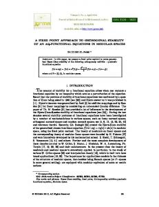
Fig. 1. Volterra prefilter equalizer.

crucial issue of choosing a signal norm in which to formulate the equalization problem. It turns out that different choices of signal norm can lead to very different theoretical performance limits. We develop a new signal norm that allows subspace information regarding response behavior of the Volterra filters to be incorporated into the analysis. In Section VI, the incorporation of subspace information into the equalizer analysis is discussed. In certain cases, this produces significant improvements in the theoretical performance bounds of the equalization algorithms, as is proved in Section VII. Specifically, the class of allowable inputs is increased, and the upper bounds on the convergence rate are improved using this information. Section VIII includes several numerical examples demonstrating these results. Conclusions are given in Section IX. II. VOLTERRA FILTER EQUALIZATION Let the space of bi-infinite real-valued sequences be denoted . An th-order Volterra filter is a polynomial mapping . If is the input to , then the output sequence is given by by

(1) are called the Volterra kernels In the equation above, of . Notice that if , then is linear. Additionally, , where is it is often convenient to write the th-order homogeneous component of . To simplify the presentation, an operator notation (e.g., ) is utilized, rather then the explicit expression of the output as in (1). models the physical system and that the Assume that desired system is also modeled as a Volterra filter. Two specific problems are studied in this paper. The first problem is prefiltering equalization. Assume that we have an input . The goal is to construct a Volterra filter so that the output of the filter in response to the prefiltered input approximates the output of the ideal filter in response to . . is called a prefilter That is, equalizer. The prefiltering problem is depicted in Fig. 1 and is formally stated as follows: 1) Given , and the input , construct a Volterra such that . Note that filter is dependent on both and . Special cases of this problem are inversion and linearization or , respectively). Applications include (i.e., loudspeaker linearization [6], [7] and channel equalization [4], [10], [12]. The second problem is postfiltering equalization. Assume that the output in response to an unknown input is observed. The goal is to construct a Volterra filter so that . is called a postfilter equalizer

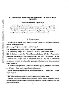
Volterra postfilter equalizer.

and depends on both and . Applications include sensor linearization and image restoration [18]. The postfiltering problem is depicted in Fig. 2 and is formally stated as follows: 2) Given , , and the output , construct a Volterra filter such that . Note that due to the nonlinear nature of and , in general, the prefilter and postfilter are different. III. SOLVING THE EQUALIZATION VIA THE CONTRACTION MAPPING

PROBLEM THEOREM

The prefilter and postfilter equalization problems are approached as fixed point problems. In general, the fixed point cannot be solved for directly. However, under certain conditions, the fixed point solution may be obtained by invoking the classical contraction mapping theorem (CMT). This is closely related to the approaches followed in [8] and [17]. Before going into the problem formulation, we briefly discuss the similarities and differences between the work in this paper and that of the previous papers. Halme et al. [8] consider the special case of the local inverse for polynomial operators on general Banach spaces, emphasizing a special construction of the local inverse. This special construction is quite different from the successive approximation construction used for the equalizers studied in this paper. The successive approximation method has two distinct advantages over the construction of Halme et al.: Theoretical upper bounds on the convergence rate of the successive approximation method are easily obtained, and the implementation complexity of the Volterra filter equalizer derived from the successive approximation scheme is generally much less. Halme et al. apply their results to solve certain types of nonlinear differential equations and to determine sufficient conditions for BIBO stability of related systems. The results surveyed by Prenter in [17] and the references therein are closer in spirit to the analysis carried out here but, again, are restricted to the special case of a local inverse. Prenter utilizes the method of successive approximation and derives conditions similar to Halme et al. for the local inverse. Prenter works with the sequence spaces and , and hence, the analysis is closer to the digital signal processing approach taken here. The survey [17] does not discuss possible applications of the results. In this section, we generalize the local inverse problem to the equalization problem at hand, and we treat the subtleties regarding the difference between the prefilter and postfilter equalization. In addition, we employ a signal processing perspective as much as possible. A. Fixed Point Formulation of Equalization Problem In this section, we derive a fixed point equation that describes both the prefilter and postfilter equalization. To do this, we need to make the following standard assumption [8], [17]:

NOWAK AND VAN VEEN: VOLTERRA FILTER EQUALIZATION: A FIXED POINT APPROACH

A1)

, which is the linear component of the filter invertible. For the prefilter equalization, we desire

, is

(2) Applying

379

In the prefilter equalization, . A fixed point

, and of

or equivalently For postfilter equalization, . The fixed point of

to both sides of (2), we have

satisfies

(9) and then satisfies

(3) Now, let

or equivalently

, and rearrange (3) as (4)

Hence, the prefilter equalization problem corresponds to the fixed point problem in described by (4). In the next section, it is shown how the fixed point can be computed using the method of successive approximation. This process of solving for leads naturally to a Volterra filter realization for the prefilter equalizer . The postfilter problem is approached as follows. Using the observed output , first compute the unknown input . This step is an inversion problem. Next, apply the desired system to . If denotes the postinverse of , then the postfilter equalizer is given by . The inverse problem is formulated as a fixed point equation similar to the prefiltering problem considered above. A neccessary condition that is an inverse is

(5) Equation (5) simply requires that the output of to must equal the original output to both sides of (5), we have

Now, let

in response . Applying

(10)

Conditions are established in the next section under which the fixed point is unique, and therefore, . Hence, solving the fixed point equation produces the unknown input , and subsequently, the desired output can be produced. B. Solving the Fixed Point Equation via the CMT One common method for characterizing solutions to fixed point problems is the contraction mapping theorem (CMT). Under certain conditions, the mapping in (8) is a contraction mapping, and the fixed point can be found by the method of successive approximation. Definition: Let be a subset of a normed space , and let be a transformation mapping into . Then, is said to be a contraction mapping if there exists an such that (11) Contraction Mapping Theorem (CMT) [13], [21]: If is a contraction mapping on a closed subset of a Banach space, there is a unique vector satisfying . Furthermore, can be obtained by the method of successive approximation, starting from an arbitrary initial vector in . If is arbitrary, and satisfies (11) for some , then the sequence , which is defined by the recursion , converges in norm to . Moreover

(6)

(12)

(7)

In order to apply the CMT to the equalization problem, the problem must be formulated on a complete, normed vector space (Banach space). Many choices of norm are possible. For example, any of the sequence norms may be chosen. For the moment, assume that we have selected a norm denoted . Define the normed vector space of sequences

, and rearrange (6) as

Under certain conditions to be established shortly, the solution of the equation above satisfies . Hence, by computing the fixed point of (7), the filter is inverted. Using the method of successive approximation to obtain and then applying to leads, naturally, to a Volterra filter realization for the postfilter equalizer . Note that both the prefilter equalization (4) and the postfilter inversion (7) are represented by the following fixed point equation: (8)

(13) is complete. In addition, we let and assume that denote the homogeneous components1 of the Volterra filter . We assume the homogeneous operators of are bounded, i.e., , and 1 The homogeneous components of the composition are easily obtained from and . Details are found in [8, Appendix C]; also see [20].

380


assume that . Details on computing bounds on these operator norms are discussed in Section V. For the equalization problem at hand, we must confirm that the mapping is a contraction mapping. This is a relatively straightforward exercise and basically follows the developments in [8] and [17]. The details are found in [15]. Here, we state the main result. First, define the contraction factor

the linear component invertibiltity assumption A1, for practical applications, we also assume finite memories. A2. and in (8) are finite memory Volterra filters. Under A2, the signals and are realized as

(14) (18)

and the polynomial (15) ensures that maps into The condition , where is the ball of radius about the origin in . The following theorem summarizes the conditions that establish the contractiveness of the equalizer. Similar results were previously derived for the special case of a local inverse in [8], [9], [16], and [17]. Theorem 1: Let be the unique positive number satisfying

If there exists

(19) of the different kernels In general, the memory lengths above may vary. For simplicity, we assume every kernel to have the same memory length . However, note that and may have different orders and respectively. The -fold iteration of the contraction mapping is realized by the following equation:

such that

(20) (16)

, and there exists a then is a contraction mapping on unique satisfying . Moreover, the sequence defined by the recursion converges in norm to for any initial and

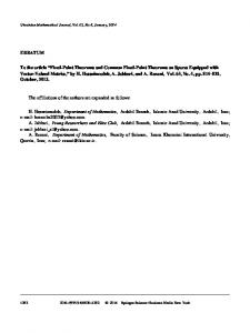
. The -fold A simple choice of initialization is equalization (20) is represented in the block diagram of Fig. 3. There are a total of Volterra filter blocks in the -fold equalizer. V. CHOOSING

(17) In the postfilter equalization problem, if , then by the uniqueness of the fixed point. In practice, the operator norms needed for the previous analysis are not easily computed. However, upper bounds on the operator norms are easily obtained (see Section V), and the statement of Theorem 1 remains the same when the norms are replaced with upper bounds [16]. Note that the condition (16) differs from similar conditions in [8], [17] because we consider the general equalization problem rather than the special case of a local inverse. Second, we have explicitly addressed both the prefilter and postfilter equalization problems. IV. REALIZING THE EQUALIZATION USING VOLTERRA FILTERS The method of successive approximation used to solve the fixed point equation (8) produces an explicit construction for the equalizing filter. The equalizer is itself a Volterra filter, and here, we define its general structure. Specifically, under certain assumptions, the -fold iteration of the contraction mapping is realized as a cascade of Volterra filters. In addition to

A

NORM

As mentioned previously, the equalization problem may be formulated using a variety of norms. In particular, any of the norms can be used. There are several reasons to carefully consider different norms. First of all, recall that to guarantee the contractiveness of the equalizer, we have the condition

where the radius bounds the norm of the signals involved. To compute , we need the operator norms . The operator norms are induced by the choice of signal norm. In practice, these induced norms cannot be computed, and we must replace the norms with computable upper bounds. The upper bounds may be tighter or looser, depending on the underlying signal norm involved. Hence, formulating the equalization problem under different signal norms produces different signal restrictions, which are necessary to guarantee the contractiveness. A second aspect of the theoretical analysis that is affected by the choice of norm is the condition that guarantees that the


Fig. 3.

equalizer

maps

into

381

-fold Volterra equalizer.

norm

:

is bounded in terms of the kernel

by (23)

This condition can be viewed in two ways. First, given an , what class of signals can be handled within this , what is the minimum framework? Alternatively, given value of so that the condition above is satsified? This can then be used to determine whether or not the mapping is contractive by computing . Either way, the choice and the upper bounds for of signal norm determines the operator norms . Because the theoretical equalizer performance depends on these quantities in a complicated nonlinear manner, it is not clear which norm will provide the most meaningful and/or illuminating results. In this section, we briefly discuss some of the benefits and limitations of different norms and propose a new norm that provides a reasonable compromise between the various choices, and that, in many cases, provides improved theoretical performance limits. A. The

and

Norms

Bounds on the operator norms for

and , respectively, are

This bound is easily obtained, and the details are found in [17]. A limitation of the norm is that it is difficult to incorporate information regarding the response characteristic of the operator into the analysis. In Sections VI and VII, response information is used to improve the theoretical performance limits. To do this, however, we need to introduce a new “window” norm that is a compromise between the norm and the norm. C. The

Norm

For (24) , and is the where Euclidean norm. It is easily verified that is a valid norm, and it can also be shown that the normed space (25)

(21) (22) denotes the -dimensional Fourier transform of the where kernel . Derivation of the operator bound is found in [17]. bound, which appears to be new, is easily obtained The using standard Fourier analysis. Note that if has finite support (i.e., finite memory), then is a continuous function on a compact set and, therefore, is bounded. This implies that operator norm is finite. the The disadvantage of the and norms is they are global measures of the signal over all time. Hence, as the signal duration increases, the total energy may increase, and consequently, so does the signal norm. The conditions of Theorem 1 that must be satisfied so that the CMT is applicable place severe restrictions on the norms of signals involved. This limits the utility of the and norms in the equalization problem. B. The

Norm

signal norm measures the maximum amplitude The of the signal and, hence, does not suffer from some of the limitations of the and norms. In this case, the operator

is complete.2 The norm has the attractive property that it only involves an length window of the signal and, hence, is local like the norm. In fact, . However, norm and like the and norms, for , unlike the the norm does reflect some of the temporal behavior of the signal. In fact, . This norm is also ideally suited to incorporate information regarding the response characteristics of the Volterra filters into the analysis. An upper bound for the operator norm is given below. The upper bound follows using standard results from Kronecker product theory, and the details may be found in [15]. Define the kernel matrix

where

.. .

.. . (26)

2 The completeness of this space is essentially established in the same manner as the completeness of is established. A proof showing that is complete is given in [13, p. 37].

382


and let be the largest singular value of the matrix . The operator norm induced by the signal norm is bounded as (27)

signal , let

, where . For the purpose of analysis, we interpret the th-order homogeneous filter as a multilinear operator and write

CMT

(30)

The predicted performance limits obtained from the basic CMT analysis of the Volterra equalization problem can be improved in many cases by incorporating subspace information regarding the Volterra filter into the analysis. If we assume that the nonlinear Volterra filter only responds to a subspace of the full input space, the class of allowable input signals is increased, and the bounds on the convergence rate are improved. Subspace response conditions such as this are often met or nearly approximated in many practical problems. A simple example that illustrates this subspace effect is the following cascade system. Consider a quadratic system defined by a linear FIR filter with vectorized impulse response followed by a squaring operation. If is the input to this system, then the output is given by

terms to reflect the output’s dependence on only the past of the input sequences . In addition, let be an rank orthogonal projection matrix, and define the seminorm3

VI. INCORPORATING SUBSPACE INFORMATION

INTO THE

(28) If we define the orthogonal projection matrix then it is easy to see that

,

(31) Note that because every

is an orthogonal projection matrix, for (32)

, and we write As in Section III, . Let be the rectangular kernel matrix defined according to (26) using the th-order kernel of . The induced operator norm is bounded, according to (27)

where is the largest singular value . For convenience, we denote this upper bound on the operator norm by

(29) is equal to the output Hence, the output in response to in response to , which is the projection of the input vector onto the space spanned by the filter vector . While this is a trivial example, the idea extends to more complicated situations. The point is that the nonlinear filter only responds to a particular subspace and produces zero output in response to inputs outside this subspace. We say that such a filter is subspace limited. More general Volterra filters may also be subspace limited. Typically, the subspace cannot be determined by simple inspection as in the example above. However, the kernel approximation and decomposition results developed in [14] allow such subspaces to be extracted from arbitrary Volterra kernels. We have shown in previous work [14] that a homogeneous Volterra filter operator is subspace limited if and only if the kernel matrix, as defined in (26), is low rank. Theorem 2 in [14] provides a method for determining the subspace for a given low-rank kernel. Efficient implementations for lowrank kernels are also discussed in [14]. These implementations are also useful for reducing the computational complexity of equalizers. VII. IMPROVEMENTS IN THEORETICAL ANALYSIS FOR SUBSPACE-LIMITED FILTERS In this section, we develop the theoretical analysis of the equalization problem under the assumption that the kernels of the Volterra filter are low rank and, hence, are subspace limited. The norm provides a convenient and practical framework for exploiting the subspace limited behavior of Volterra filters. To simplify the notation, for any

(33) The following lemma characterizes a subspace limited Volterra and will be filter in terms of the kernel matrices used in the subsequent analysis. Lemma 2: Let be an rank orthogonal projection matrix. If for any unitarily invariant matrix norm

then for every set of signals (34) Furthermore (35) Lemma 2 follow easily from previous results regarding lowrank kernel matrices established in [14], and the details are given in [15]. Before stating the convergence results for a subspace limited equalizer, define the contraction factor

and let

With this notation in place, we state the following theorem. 3 A seminorm satisfies all properties of a norm except that its value may be zero for nonzero signals [13].


383

Theorem 2: Let be the unique positive number satisfying . If for some orthogonal projection matrix i) , such that , ii) there exists then there exists a unique satisfying , or equivalently, . Furthermore, the sequence defined by converges in norm to for any and

The proof of Theorem 2 is very similar to the proof of Theorem 1. The only difference is that Lemma 2 and (32) are used in some of the steps in a straightforward way. Again, the details can be found in [15]. Comparing the statements of Theorems 1 and 2, the obvious question arises. What do we gain by exploiting the subspace limited condition? There are two distinct improvements gained by incorporating prior knowledge of subspace limited behavior: • guaranteed equalizer convergence for a larger set of input signals , • tighter bounds on the rate of convergence. In the appendix, we discuss the details of these two points and establish that by exploiting prior information (the subspace limited behavior of ) we are able to guarantee equalizer convergence for a larger class of problems. We also show that incorporation of prior information results in tighter bounds on the error performance of the equalizer in all cases.

Fig. 4. Saturation nonlinearity.

curve in Fig. 4. The saturation characteristic is defined by the cubic polynomial (37) . The dotted line in Fig. 4 where, in this case, shows the linear component of this nonlinearity for comparison. For this example, assume that the input is unknown and that the nonlinear system is known. The goal is to recover the original input using only the observed output . In this case, because of the simple form of the nonlinear system, we could directly recover . However, to illustrate the methods of this paper, we apply the CMT. Using the notation developed in Sections II and III, the nonlinear system is given by (38)

VIII. NUMERICAL EXAMPLES

is a linear FIR filter whose impulse response is and where is a cubic Volterra filter whose 3-D kernel is given

where

In this section we examine two numerical examples that demonstrate the equalization methods and, in particular, highlight the use of Theorem 2. In the first example, we simulate a signal recovery problem that is posed as a postfilter equalization. The second example illustrates a prefilter equalization scheme. Both examples assume that we have a Volterra filter model of the physical system that is to be equalized. This Volterra filter explicity defines the equalizing filter as established in Section IV. The equalization filter used in our simulations is implemented as the cascade Volterra filter structure depicted in Fig. 3. In practice, the Volterra filter model of the physical system would first be identified or deduced by other means. A. Example 1: Postfilter Equalizer In this example, we consider the following problem. A sinusoidal process (36) is the input to a nonlinear system given by the cascade of a linear FIR filter with impulse response followed by the memoryless nonlinear saturation characteristic depicted by the solid

(39) denotes the th element of . The best linear where filtering solution to this problem is to filter the output with the inverse of the linear FIR filter . In this case, an approximate linear inverse filter has the impulse response . produces a Applying the inverse to the observed output signal , where, again, we are using the notation previously developed for the postfilter equalization (see Section III). The true input and the residual error of the linear inverse filtering are shown in Fig. 5. The maximum amplitude of the residual error is roughly 5% of the input amplitude, and a better estimate of the original input may be obtained using nonlinear processing. We will formulate the problem using the and norms.4 The norm is convenient for this case because the cubic filter has a memory length of 5. The contraction mapping in this case is

4 Note that due to the periodicity of the input signal, the signals involved are and norms are not applicable. not finite energy signals, and hence, the

384


TABLE I POSTFILTER EQUALIZER CONVERGENCE Actual Theory

0.0653 0.0653

0.0092 0.0279

0.0014 0.0156

0.0002 0.0098

Fig. 5. Original input and linear equalizer error.

Initializing the contraction at gives the linear inverse solution. That is, . The hope is that by iterating the mapping to obtain , , and so on, better and better approximations to the original input are obtained. First, we will examine the formulation. To theoretically guarantee the convergence of the iteration, the conditions of Theorem 1 must be satisfied. The upper bound (23) on induced norm of the cubic filter is . Next, solving for , the positive number satisfying (40) produces produces

. Substituting into the expression for . Unfortunately, in this problem (recall ), and hence, Theorem 1 cannot be applied. Next, we formulate the problem using the norm. The upper bound (27) for the induced operator norm is , which, in this case, leads to . However, , and again, the conditions of Theorem 1 are not met! Fortunately, the fact that is subspace limited can be exploited, and Theorem 2 can be successfully applied. To see this, first consider the SVD of the kernel matrix corresponding to . In this case, the singular values are . Because the kernel matrix is rank 2, we can deduce that the cubic filter is subspace limited. Letting be the orthogonal projection onto the subspace spanned by the two right singular vectors corresponding to the two nonzero singular values of , we have for all unitarily invariant matrix norms. Therefore, Lemma 2 is satisfied. Using this projection and the corresponding seminorm , we have , and since , Theorem 2 may be applied! In and fact, solving for the that satisfies substituting the solution into the expression for the theoretical contraction factor produces (41) which is an upper bound on the convergence rate in this case. Table I shows the theoretical and actual convergence norm sense. Recall that behavior of this equalizer in the is the output of the linear equalizer, and for ,

Fig. 6. Errors of linear and Volterra equalizers.

. The actual computation of the fold equalization is performed using the cascade Volterra filter structure depicted in Fig. 3. That is, is simply the output of the equalizing filter pictured in Fig. 3 in response to the input signal . Notice that the theory does overbound the actual performance. For example, the theoretical bound on the error is a factor of 3 larger than the actual error. However, the theoretical bounds may provide guidelines that allow one to quantify the tradeoff between equalizer complexity and performance. The residual errors of the linear equalizer , one iteration Volterra equalizer , and two iteration Volterra equalizer are depicted in Fig. 6. The theory, even when subspace information is incorporated, does not guarantee equalizer convergence for saturations much more severe than the one in the previous example. However, in practice, much more demanding problems can be tackled using the successive approximation approach. As an example, consider the same nonlinear system structure with a more severe saturation characteristic (42) This saturation is depicted in Fig. 7. Computing the necessary Volterra filters and implementing the equalizer, we obtain the following actual convergence behavior shown in Table II. It appears that the equalizer is converging; however, this convergence cannot be theoretically guaranteed using any of the norms discussed in this paper. This example demonstrates the limitations of the existing theory. For this case, the residual errors of the linear equalizer , one iteration Volterra equalizer , and four iteration Volterra equalizer , are depicted in Fig. 8. B. Example 2: Prefilter Equalizer In this example, we consider the following equalization problem. A pulse input , which is shown in Fig. 9, is applied


Fig. 7.

385

Fig. 9. Input and output of quadratic system.

Severe saturation nonlinearity.

TABLE II POSTFILTER EQUALIZER CONVERGENCE Actual

0.1562

0.0796

0.0493

0.0338

Fig. 10.

Fig. 8.

Errors of linear and Volterra equalizers—Severe saturation.

to a nonlinear filter defined by (43) is a quadratic Volterra filter with memory . where The output is also shown in Fig. 9. The quadratic kernel associated with is given by the outer product of the vector

with itself and is designed to represent a lowpass quadratic effect. The kernel is depicted in Fig. 10. The goal is to predistort the input pulse so that the output of the nonlinear filter is the desired pulse . We will analyze this equalization problem using both the and norms. The contraction mapping in this case is (44) norm. The First, we analyze the equalization using the upper bound (23) on the induced norm of the quadratic filter is . Next, solving for , the positive number satisfying (45)

Quadratic filter kernel.

produces . Substituting into the expression for produces . For the unit amplitude pulse input, we have . Hence, , and Theorem 1 cannot be applied. In addition, although this signal is of finite duration, working with the or norm fails to guarantee convergence as well. If we formulate the problem using the norm and incorporate the exploit the fact that is subspace limited, then the following bounds on the convergence are obtained. First, let be the square kernel matrix associated with the quadratic filter . In this case, the kernel matrix is rank with single nonzero singular value 0.05. Let denote the projection onto the subspace spanned by the associated singular vector. Using the norm, we compute . The subspace seminorm of the input is and comparing this with shows that Theorem 2 may be applied. Solving for the that satisfies and substituting the solution into the expression for the theoretical contraction factor produces (46) which is an upper bound on the convergence rate in this case. The output errors with no equalization, one iteration of the Volterra equalizer, and two iterations of the Volterra equalizer are depicted in Fig. 11. Table III shows the theoretical and actual convergence of behavior of this equalizer in the norm sense. In this case, , which is the original input, and for . Theoretically, convergence cannot be guaranteed if the gain is increased. However, as in the of quadratic component postfiltering example, the actual performance limits are less

386


Fig. 11.

Fig. 13.

Errors of Volterra equalizers.

TABLE IV PREFILTER EQUALIZER CONVERGENCE

TABLE III PREFILTER EQUALIZER CONVERGENCE Actual Theory

0.1892 0.1892

Fig. 12.

0.0281 0.0892

0.0030 0.0520

Errors of Volterra equalizers—Strong quadratic nonlinearity.

0.0003 0.0333

Input and output—Strong quadratic nonlinearity.

restrictive. The same problem is simulated again, this time with the singular value of equal to 0.2, which is four times larger than the previous case. The input and output of this system are shown in Fig. 12. Table IV demonstrates that the first few iterations of the equalizer are tending toward a fixed point. Fig. 13 shows the original output error with no equalization, the error using one iteration of the Volterra prefilter equalizer, and the error using four iterations of the equalizer. It is clear from Fig. 13 that the equalizer is accomplishing the desired filtering. IX. CONCLUSION Theoretical convergence of a large class of nonlinear equalization problems is examined. The systems and equalizers studied here are modeled as Volterra filters, and the equalization problem is formulated as a fixed point problem. Conditions under which the fixed point equation is a contraction mapping are established. The method of successive approximation results in an equalizer that can be realized as a cascade of simple, repeated, Volterra filters. To guarantee convergence of the equalizers, constraints on the norms of the involved signals are obtained in terms of the operator norms of the associated Volterra filters. The

Actual

0.7570

0.4286

0.2181

0.0958

convergence analysis and resulting bounds on the rates of convergence depend on these norms in a complicated and nonlinear manner. Hence, formulating the problem under different norms may produce quite different theoretical bounds on the convergence behavior. The benefits and limitations of various signal norms are discussed, and the “window” norm is introduced. We demonstrate how knowledge that the Volterra filter only responds to a subspace of the full input signal space can be incorporated to improve the theoretical analysis of equalization algorithms. Theoretical norm analysis exploiting subspace information and the indicates that the class of allowable inputs and the upper bounds on the convergence rate are improved. Several examples of prefilter and postfilter equalization problems are presented. In two cases, it is shown that convergence is guaranteed using subspace information and the norm when formulations based on traditional signal norms fail to guarantee convergence. Other simulations show that the theoretical analysis is overly conservative in many cases. This suggests that further study is still needed to better understand the nonlinear equalization problem. Our experience has led us to the following practical guideand are most useful in practice since lines. First, the and norms often fail to guarantee convergence as the the signal duration increases. It is important to note, however, that for finite duration signals all norms are equivalent, and hence, convergence in one norm will guarantee convergence in other senses. In practice, one may simply implement the equalizing filter described in Section IV and evaluate the performance. As the examples demonstrated, the equalizers often work very well even when the convergence cannot be absolutely guaranteed. In practice, it may not be possible to guarantee convergence; however, the analysis presented here leads to equalization filters that may provide very good results. There are several avenues for future work here. First, the initial work exploiting subspace information may be expanded and improved. In addition, such information may be useful in equalization schemes that are not based on a contraction


mapping approach. For example, subspace information may be used to improve the performance of adaptive Volterra equalizers based on mean-square error criteria. Another very important open problem is the issue of noise. In real systems, noise is usually present. Our analysis here is a purely deterministic approach, and it is crucial to incorporate the effects of noise for many problems of practical interest. We are currently addressing these and other issues in ongoing work.

387

, where for all by contradiction. Suppose equivalently,

Multiplying both sides by

. Now, we proceed or,

, we have

APPENDIX A IMPROVEMENTS OBTAINED VIA SUBSPACE-LIMITED ANALYSIS As mentioned in Section VII, there are two distinct improvements gained by incorporating prior knowledge of subspace limited behavior. First, the subspace limited condition (assumption i) in Theorem 2) increases the set of for which the problem can be solved (via CMT). To see this, notice that ii) in Theorem 2 requires an satisfying , whereas the corresponding condition in Theorem 1 requires to satisfy . Since and since is increasing on , it follows that a larger class of signals is admissible under the subspace limited assumption. In other words, if , then but not necessarily vice versa. Second, for fixed , incorporating the subspace limited assumption can improve the bound on the convergence rate. To see this, consider the following argument. Recall that is the unique positive number satisfying . It is also on on , easily verified that and . Hence, is the maximum of on . Let be defined as the positive real number for which . If , then Theorems 1 and 2 hold. If , then Theorem 1 does not apply, and Theorem 2 . Define . applies if and only if to be arbitrary, With this notation in place, take and define to be the unique number in solving . We interpret the number as the smallest feasible of Theorem 2 with . In the following theorem, we consider the contraction factor as a function of . Theorem 3: is an increasing function of on . Furthermore, if , then . Proof: To prove the first statement, recall that on and . Hence, as increases, so does . Therefore, is strictly increasing on . Then, note that on . It follows is increasing on . that To prove the second statement, notice that by rearranging , we have

It follows that has a power series representation , where for all . Now,

This implies , which in turn implies that since , and hence, we have a contradiction. The significance of Theorem 3 is this: Assume that satisfies the hypothesis of Theorem 1. If, in addition, is subspace limited, in the sense of i) in Theorem 2, and if , then the upper bound on the contraction factor is decreased by at least a factor of compared with the standard CMT bound without incorporating the subspace limited condition. Two other observations can be deduced from Theorem 3. First, if , then we have one-step convergence (i.e., take to be any signal satisfying , e.g., .) Second, with a slight modification of Theorem 3, if , then for . In particular, if , which is an th-order homogeneous filter, then . REFERENCES [1] O. Agazzi, D. G. Messerschmitt, and D. A. Hodges, “Nonlinear echo cancellation of data signals,” IEEE Trans. Commun., vol. 30, pp. 2421–2433, 1982. [2] E. Bilglieri, A. Gersho, R. D. Gitlin, and T. L. Lim, “Adaptive cancellation of nonlinear intersymbol interference for voiceband data transmission,” IEEE J. Selected Areas Commun., vol. JSAC-2, pp. 765–777, 1984. [3] J. W. Brewer, “Kronecker products and matrix calculus in system theory,” IEEE Trans. Circuits Syst., vol. CAS-25, pp. 772–781, 1978. [4] D. D. Falconer, “Adaptive equalization of channel nonlinearities in QAM data transmission systems,” Bell Syst. Tech. J., vol. 57, no. 7, pp. 2589–2611, 1978. [5] G. Folland, Real Analysis. New York: Wiley, 1984. [6] W. Frank, R. Reger, and U. Appel, “Loudspeaker nonlinearities—Analysis and compensation,” in Proc. 26th Asilomar Conf. Signals, Syst., Comput., Oct. 1992. [7] F. Gao and W. M. Snelgrove, “Adaptive linearization of a loudspeaker,” in Proc. ICASSP, 1991, pp. 3589–3592. [8] A. Halme, J. Orava, and H. Blomberg, “Polynomial operators in nonlinear systems analysis,” Int. J. Syst. Sci., vol. 2, pp. 25–47, 1971. [9] A. Halme and J. Orava, “Generalized polynomial operators in nonlinear systems analysis,” IEEE Trans. Automat. Contr., vol. AC-17, pp. 226–228, 1972. [10] R. Hu and H. M. Ahmed, “Echo cancellation in high speed data transmission systems using adaptive layered bilinear filters,” IEEE Trans. Commun., vol. 42, nos. 2/3/4, 1994. [11] A. J. M. Kaiser, “Modeling of the nonlinear response of an electrodynamic loudspeaker by a Volterra series expansion,” J. Audio Eng. Soc., vol. 35, no. 6, 1987. [12] G. Lazzarin, S. Pupolin, and A. Sarti, “Nonlinearity compensation in digital radio systems,” IEEE Trans. Commun., vol. 42, nos. 2/3/4, pp. 988–998, 1994. [13] D. G. Luenberger, Optimization by Vector Space Methods. New York: Wiley, 1968.

388


[14] R. Nowak and B. Van Veen, “Tensor product basis approximations for volterra filters,” IEEE Tran. Signal Processing, vol. 44, pp. 36–51, Jan. 1996. [15] R. Nowak, “Volterra filter identification, approximation, and equalization,” Ph.D. dissertation, Dept. Elect. Comput. Eng., Univ. of WisconsinMadison, 1995. [16] J. Orava and A. Halme, “Inversion of generalized power series representation,” J. Math. Anal. Applicat., vol. 45, pp. 136–141, 1974. [17] P. M. Prenter, “On polynomial operators and equations,” in Nonlinear Functional Analysis and Applications. New York: Academic, 1971, pp. 361–398. [18] B. E. A. Saleh, “Bilinear transformations in optical signal processing,” SPIE, vol. 373, 1981. [19] M. Schetzen, “Theory of th-order inverses of nonlinear systems,” IEEE Trans. Circuits Syst., vol. 23, no. 5, pp. 285–291, 1976. [20] M. Schetzen, The Volterra and Wiener Theories of Nonlinear Systems. New York: Wiley, 1980. [21] E. Zeidler, Nonlinear Functional Analysis and Its Applications I: FixedPoint Theorems. New York: Springer-Verlag, 1986.

Robert D. Nowak (S’89–M’95) received the B.S. (with highest distinction), the M.S., and the Ph.D. degrees in electrical engineering from the University of Wisconsin, Madison, in 1990, 1992, and 1995, respectively. He held a Wisconsin Alumni Research Foundation Fellowship while working on the M.S. degree. He has also worked at General Electric Medical Systems. While working towards the Ph.D. degree, he was a Rockwell International Doctoral Fellow. In 1995 and 1996, he was a Research Associate at Rice University, Houston, TX. He is currently an Assistant Professor of Electrical Engineering at Michigan State University. His research interests include statistical and nonlinear signal processing, image processing, and related applications.

Barry D. Van Veen (S’81–M’86) was born in Green Bay, WI. He received the B.S. degree from Michigan Technological University, Houghton, in 1983 and the Ph.D. degree from the University of Colorado, Boulder, in 1986, both in electrical engineering. He was an ONR Fellow while working on the Ph.D. degree. In the spring of 1987, he joined the Department of Electrical and Computer Engineering at the University of Colorado. Since August, 1987, he has been with the Department of Electrical and Computer Engineering at the University of Wisconsin, Madison, where he is currently an Associate Professor. His research interests include signal processing for sensor arrays, spectrum estimation, adaptive filtering, and biomedical applications of signal processing. Dr. Van Veen was a recipient of the 1989 Presidential Young Investigator Award and the 1990 IEEE Signal Processing Society Paper Award.