VOLUME DECOMPOSITION AND FEATURE RECOGNITION FOR HEXAHEDRAL MESH GENERATION* Yong Lu1, Rajit Gadh2, Timothy J. Tautges3 1
Ph. D. Student, I-CARVE Lab, University of Wisconsin-Madison,
[email protected], http://smartcad.me.wisc.edu/~yong 2
Associate Professor, I-CARVE Lab, University of Wisconsin-Madison,
[email protected], http://smartcad.me.wisc.edu/~gadh 3
Sandia National Laboratories, tjtautg@sandia,gov, http://endo.sandia.gov/9225/Personnel/tjtautg
ABSTRACT Considerable progress has been made on automatic hexahedral mesh generation in recent years. Several automatic meshing algorithms have proven to be very reliable on certain classes of geometry. While it is always worth pursuing general algorithms viable on more general geometry, a combination of the well-established algorithms is ready to take on classes of complicated geometry. By partitioning the entire geometry into meshable pieces matched with appropriate meshing algorithms, the original geometry becomes meshable and may achieve better mesh quality. Each meshable portion is recognized as a meshing feature. This paper, which is a part of the feature based meshing methodology, presents the work on shape recognition and volume decomposition to automatically decompose a CAD model into meshable volumes. There are four phases in this approach: Feature Determination to extract decomposition features, Cutting Surfaces Generation to form the “tailored” cutting surfaces, Body Decomposition to get the imprinted volumes, and Meshing Algorithm Assignment to match volumes decomposed with appropriate meshing algorithms. The feature determination procedure is based on the CLoop feature recognition algorithm that is extended to be more general. Results are demonstrated over several parts with complicated topology and geometry. Keywords: mesh generation, hexahedral meshing, feature recognition, volume decomposition, solid modeling
1. INTRODUCTION The Finite Element Analysis (FEA) technique is widely used for parts prototyping and design verification. Meshing, the procedure to prepare FEA model, proves to be time-consuming and error prone. The automation of *
mesh generation can immediately speed the product design cycle. Automatic meshing generation on tetrahedral elements has achieved much success and there are a few reliable tetrahedral meshing algorithms available nowadays. FEA on Hexahedral elements uses higher order interpolation functions and tends to achieve more accurate results. Hexahedral mesh is preferable to tetrahedral mesh
This work was funded by Sandia National Laboratories, operated for the US DOE under contract No. DE-AL0494AL8500. Sandia is a multi-program laboratory operated by Sandia Corporation, a Lockheed Martin Company, for the U.S. DOE.
in some applications for several reasons [1]. Many researchers have been investigating algorithms to automate the procedure to get all-hexahedral elements model [2]. Although significant progress has been made over the years, the completely automated method that is demanded by designers who practice FEA is not yet available due to the general difficulty of filling hexahedral elements into 3D space. Meshing is a process of spatial decomposition. A physical 3D space is decomposed into small elements with required topology and geometry constraints. Different algorithms differ in the way that they decompose the 3D space. Many hexahedral-meshing algorithms are suggested. There are mapping/sub-mapping algorithm [3] [4], Sweeping [5] [6], Plastering [7], Whisker Weaving [8], shrinking-mapping method [9], and Grid based method [10] [11], etc. Human experience of meshing procedure may shed some light on the automatic meshing algorithms that we are pursuing. It is certainly worthwhile to go on developing general automatic algorithms like plastering and whisker weaving to deal with general geometry directly. In the meantime, it is also valuable to pursue a decompositionbased meshing methodology that mimics the human procedure of meshing: decompose the original geometry globally and make full use of meshing solutions available. Although mapping, submapping and sweeping work on constrained geometry, they can usually deal with a large portion of practical parts. The working versions of plastering and whisker weaving also become reliable on certain classes of difficult geometry. In another view, the complexity of the geometry and topology of the original model is reduced by decomposition, thus the model becomes meshable with well established approaches. Besides improving the meshability of a model, the quality of mesh can be enhanced and the meshing time can be reduced. The complicated meshing algorithms that take on more versatile geometry are more computationally expensive than simpler ones. For example, the meshing speed of whisker weaving is 100 hexahedral elements per second, while the speed of mapping is 10,000 hexahedral elements per second [12][13]. Through decomposition, the geometry and topology of the volumes usually become simpler, thus it is possible for them to be meshed by algorithms like sweeping and mapping/sub-mapping, which generally produce fast and good quality mesh. Generally, computationally inexpensive meshing algorithms that minimize meshing time but maximize mesh quality can be chosen on volumes decomposed. This paper is to report the progress that we made on the feature based decomposition approach [12] [16] [17] [18]. Other meshing algorithms based on decomposition have been developed recent years. ICEM AutoHexa is an objectbased hexahedral mesher [19]. The medial axis transform (MAT) technique is suggested for decomposition and meshing [20] [21] [22]. Sheffer et al. [23] propose the Embedded Voronoi Graph to guide decomposition. Chiba et al. [24] introduce an automatic hexahedral mesh generation method based on the shape-recognition and boundary-fit algorithms. Bih-Yaw Shih and Hiroshi Sakurai present a mesh generation tool via swept volume
decomposition [25]. The algorithms above have their advantages in their own courses, but also have their limitations. This paper employs Feature Recognition (FR) technique to guide the decomposition in an intelligent way, which attempts to obtain decomposition results intuitive to meshing.
2. FEATURES, VOLUME DECOMPOSTION, AND MESHING Feature Recognition (FR) is the procedure to extract design or manufacturing features from a solid model. It is widely used in design and manufacturing. Extensive research has been performed in FR field [26] [27] [28]. Usually FR technique is domain-dependent. When using FR technique in the meshing domain, different requirements are enforced.
2.1 Features Traditionally FR techniques are developed in the domain of design and manufacturing. Usually they are domaindependent and not suitable to serve as a feature determination algorithm for the purpose of meshing [18]. Generally only sets of feature primitives relevant to the application are recognized. They may only represent a small portion of the whole part. “Bosses”, “ribs”, “slots” and “key-ways” are defined based on different requirements for design and manufacturing functionality. The major portion of the part may be left with no further recognition. The features defined may not be rational for meshing. For FR in the machining domain, “boss” or “rib” is determined because of the different functionalities. In meshing, they are regarded as the same feature as long as the same algorithm can be used to mesh them. Negative features have no direct value to meshing. In the meshing domain, only exclusive addition operation is well recognized and implemented. Negative features or a set of features having overlapping volumes are not acceptable in the meshing domain. The meshing feature decomposer takes a solid model as the input and outputs recognized meshing features. These meshing features are sub-volumes matched with appropriate meshing algorithms. Among them, there are sweeping features, mapping/sub-mapping features, plastering features, Whisker Weaving features, etc. The procedure is shown in Fig. 1. Swept along this direction Meshing Feature Decomposer
Swept along this direction
A Solid Model Meshing Features
Figure 1. Meshing Feature Decomposer The feature recognition technique to be used for the purpose of meshing should be flexible enough to
accommodate meshing features. It is not necessary to be a recognizer at the high end of an application, thus it may not be tightened with the specific application and can be easily adjusted to meet the needs of the meshing domain. Most decomposition takes place at concave transition zones. A fundamental and convexity-aware FR technique may serve the purpose of the decomposition for meshing well.
CLoops are used to define four classes of shape: Protrusion, Blind Depression, Through Depression, and Bridge [17].
Among so many feature recognition techniques, CLoop based FR technique [16] [17] [18] [29] is chosen as the foundation of the feature decomposer for meshing. This paper uses the feature recognition technique extended from the CLoop concept in the general feature determination phase. The CLoop feature is addressed in the following sub-section. Figure 2. PLoop, HLoop and SLoop
2.1.1 CLoop Feature Gadh and Prinz suggested an abstraction of CLoop for feature recognition and CLoop was introduced as a closed set of linked edges with the same convexity [29]. The CLoops, combined with rules, are used to extract both protrusive features like ribs, bosses, etc. and depressive features like holes and slots. For the purpose of decomposition, Liu and Gadh extended the definition of CLoop to be an open or closed link of edges by introducing PLoop and HLoop [16] [17]. The concept of PLoop and HLoop is relaxed further and SLoop, a type of CLoop with mixed convexity, is introduced to accommodate more classes of features such as fillet shapes [18]. An edge can be classified as Concave Edge, Convex Edge, Neutral Edge and Hybrid Edge based on the edge angle [17] [18]. Based on the convexity of edges, a CLoop is classified as [17] [18]: • Pure CLoops. Pure CLoop, denoted as λp, is a closed link of edges with the same convexity. It can be further classified as Pure Concave CLoop; Pure Convex CLoop; Pure Neutral CLoop [18]. For simplicity, we refer to Pure CLoop as PLoop. • Pseudo CLoop. Pseudo CLoop, denoted as λs, is a closed link of edges with mixed convexity. The edges in the CLoop can be neutral, concave, convex or hybrid. For simplicity, we refer to Pseudo CLoop as SLoop. • Hybrid CLoop. Hybrid CLoop, denoted as λh, is an open link of edges with the same or mixed convexity. For convex and hybrid edges, the similar geometric constraints are enforced as SLoop to ensure that a limited set of hybrid CLoops, which are suitable for decomposition, is formed. For simplicity, we refer to Hybrid CLoop as HLoop. Fig.2 illustrates the three different kinds of CLoop. The inclusion of SLoop and extension of PLoop and HLoop allow for the definition and extraction of more decomposition features that can not be determined by the previous definition of PLoop and HLoop.
Meshing features are protrusive volumes. Shapes such as protrusion and bridge are recognized for decomposition. A bridge feature is converted to a protrusion feature when the adjacent protrusion feature is cut off. In practice, it is not necessary to distinguish a protrusion from a bridge. Negative features are not decomposed for meshing. However, recognition on depressive volumes can give some guidance in some phases of our approach.
2.1.2 Meshing Features The ultimate goal of the meshing feature recognition is to get meshable sub-volumes. These sub-volumes, when matched with appropriate meshing algorithms, become meshing features. The “appropriate” meshing algorithm by default means the most computationally inexpensive algorithm that can retain the satisfying mesh quality. It can change to the algorithm with the best mesh quality or with the fast meshing speed based on the requirement of certain application context. CLoop based FR
Volume Decomposition
Meshing Algorithm Assignment
Solid Model Meshing Patterns based FR
Volume Decomposition
Meshing Features
Figure 3. Retrieving Meshing Features There are two ways to retrieve meshing features, as shown in Figure 3. One is to begin with CLoop based feature recognition and decomposition and then assign suitable meshing algorithms to decomposed volumes; the other is to directly use meshing patterns to guide the recognition and decomposition from the beginning. The direct way could guarantee the volumes decomposed are suitable for meshing. Besides, it allows for the extraction of some decomposition features that can not be defined by the CLoop. Its disadvantage is that the matching patterns of those meshing features are more complicated and some of them are even ambiguous. Decomposition directly with meshing features is more computationally expensive. In
addition, it is not expected that all portions of the model could be matched with an automatic meshing schema. In this sense, even if the volumes decomposed by the CLoop is not good for automatic meshing algorithms, it is still good to cut off because generally the decomposition is helpful for manual meshing. Thus, the decomposition strategy is designed to respond to the considerations above while making reasonable attempts to achieve the possibly best decomposition result. The process begins with CLoop based decomposition and the knowledge of meshing patterns is used to guide the selection of the cutting loops and the generation of cutting surfaces. Then for the leftovers where no CLoop can be found and no automatic meshing algorithm may be assigned, meshing patterns are used directly to guide further decomposition. Among many available meshing algorithms, the matching patterns for sweeping, mapping and sub-mapping are easy to abstract. But usually for many other meshing algorithms, the topological and geometric requirement is not obvious and matching patterns for them can be difficult to abstract. A matching pattern of a meshing algorithm has the nature of changing along with the advance of the meshing algorithm itself. Meshing patterns need to be adjusted along with the progress of the meshing algorithms.
2.2 Volume Decomposition We have Ω as the operator representing the entire decomposition procedure to obtain meshing features. B represents the original body. W is the decomposition set that holds all the decomposed volumes including the intermediate results generated during the decomposition procedure. Then we have:
Ω ( B) = W
(1)
V is the set of volumes ultimately left at the end of decomposition for meshing and
vi ∈ V
i ∈ [1, n]
(2)
if each volume v can be matched with an automatic meshing algorithm. But it will always hold true if we relax it by introducing the manual algorithm as a candidate. To measure the success of decomposition for meshing, we introduce φas the automatic meshing ratio. φis the ratio of the volume that can be meshed automatically to the entire volume of the original body, thus:
φ = V (M )
(6)
V ( B)
where V is the operator to calculate the volume. There are some decomposition algorithms proposed in the domains of computational geometry and feature recognition [30] [31] [32] [33]. Chazelle introduced the technique to decompose non-convex objects into convex components [30], but the shapes of volumes decomposed can be arbitrary and the algorithm doesn’t recognize the rationale of finite element meshing. Woo suggested the process called ASV (Alternating Sum of Volumes) [31]. Hiroshi presented the abstraction of “maximal volumes” [32] [33].
2.2.1 Volume Decomposition Strategies It is natural to represent the decomposition procedure as a tree, called a decomposition tree. The root of a decomposition tree is the original model B. The set of nodes except the root in the decomposition tree is set W and the set of leaf nodes is set V. Specially, we call the evolution of a node to produce its children nodes as a “split”.
Di
D0 = B
S
Di + 1 = S ( Di )
Di+1
V = Dn
Figure 4. Recursive Decomposition
Then
v i ⊆ B,
vi ∩ v j = φ
We refer to a bounding loop that is used to generate cutting surfaces for decomposition as a “separator”. Separators are formed after CLoops or meshing features are recognized.
i ∈ [1, n] i, j ∈ [1, n]
(3)
n
B = ∑ vi i =1
where ∑ is the operator of exclusive addition. M is the set of meshing features and Ψ is the operator of the meshing algorithm assignment, then
Ψ (V ) = M
(4)
We hope n
B = ∑ m i , mi ∈ M i =1
(5)
The decomposition procedure is recursive. As shown in Figure 4, the output of the operator S, which represents the decomposing operation based on the separators, is sent back to the operator as the input. The operation stops when no separator is available. Usually multiple separators are found to decompose a volume. If the separators are consumed one at a time for a “split”, the decomposition tree is a binary tree. If more than one can be consumed for a “split”, the resulting decomposition tree is a general tree. These are two different decomposition strategies. We call the former binary decomposition and the latter non-binary decomposition. In a binary decomposition, a single separator is chosen from all the available separators to achieve the best cutting result at that stage. New separators could be uncovered
from each new volume. The new ones together with old ones form the pool where the separator for next cutting is chosen.
Solid Model
CLoop or Meshing Pattern based FR
Any cuttable separators
No
Yes
I
Cutting Surfaces Generation II
Volume Decomposition
III
No
Meshing Features Determination Yes
Figure 5. Binary Decomposition
Auto Mesher
In a non-binary decomposition, among the available separators, all of the “cuttable” separators are used to decompose the model. The old “un-cuttable” separators may become “cuttable” on the new volumes and new separators could be found on them too. Then, both new and old separators of every volume are used to further decompose the volume.
Figure 7. Feature Decomposition Procedure The decomposition procedure is shown in Figure 7.
2.2.3 Knowledge based Decomposition Meshing Patterns or CLoop based FR
I
Manual Mesher
Meshing Patterns
Cutting Surfaces Generation
Heuristic Rules
II
An Auto-meshing Method Assigned?
III
Figure 6. Non-binary Decomposition Figure 5 and Figure 6 show different decomposition trees that result from the two different decomposition strategies. The problems of separator cuttability and comparison are to be addressed later.
2.2.2 the Steps of Volume Decomposition There are four phases in our approach for CLoop based volume decomposition: CLoop based feature recognition, cutting surfaces generation, volume decomposition and meshing features determination. For the volume decomposition approach based directly on meshing features, there are three phases: meshing features determination, cutting surfaces generation and volume decomposition.
Volume Decomposition
Figure 8. Knowledge Based Feature Decomposition Volume decomposition is a procedure where artificial intelligence should be applied. The feature-based algorithm is an attempt to do decomposition in an intelligent way. We are trying to mimic the way that a meshing expert would handle a model that could not be meshed automatically in the beginning. The expert may try to decompose it into several portions, each of which can be matched with a known meshing template that either could be easily meshed manually or is suitable for an available auto-meshing tool. This procedure requires considerable knowledge of meshing algorithms and decomposition tools. Even an expert may experience several trials and failures before finding the best solution but usually an acceptable one in practice to manipulate the geometry.
The knowledge consists of the understanding of the meshing templates that come from the available meshing algorithms and generally are constrained topologically and geometrically. It includes some rules, heuristic in nature, to guide the decomposition. Nearly every phase of the feature decomposition needs the guidance from the knowledge, as illustrated in Figure 8.
End Mark n with “finished” flag. Remove n from the list L. Function end. List Ψ holds all PLoop in the model M.
3.2 Determination of SLoop 3. DETERMINATION OF CLOOP AND CUTTABLE SEPARATORS CLoop determination is a procedure of graph searching. Both PLoop and SLoop are a closed link of edges, while HLoop is an open link of edges. The search of PLoop and SLoop is very similar except for the different requirement on convexity. We define G(e) as the edge graph of model M. A CLoop is formed by linking edges sharing the required convexity in the Graph G.
3.1 Determination of PLoop Every edge can be marked with a flag “unmarked”, “in progress” or “finished”. L is a list of edges. λis a list of edges which represents a CLoop. Ψ holds a list of CLoops in the model M. Begin with an edge graph G (e) Start with initializing all nodes of concave edges by marking them with flag “unmarked”. Initialize an empty list Ψ . Initialize an empty ordered list L . For every node of a concave edge e that is “unmarked” Do depth-first search by calling DFS (e). Depose the list L. End For End Function DFS (n) Mark n “ in progress” Put n in list L. For every successive node of concave edge m of n (Successive nodes are all the adjacent nodes of node n except the node preceding n in the traversal path.) Begin If m is “unmarked”, then do DFS (m). Else if m is marked with “in progress” then Initialize an empty list λ. Copy nodes in L from m through n into list λ. Put λinto list Ψ . Else if m is marked with “finished” then Do nothing. End if.
In essence, the procedure to determine SLoop is the same as PLoop. The only difference is that there is a different requirement on edge convexity in the loop. A Sloop is formed by edges with different convexity. SLoop can define some features that are impossible to define by CLoop and HLoop. For example, they can be used to determine a fillet-type feature. As shown in Figure 2, two SLoops are extracted. One of them bounds a fillettype shape.
3.3 Determination of HLoop HLoop is an open CLoop and one more step is needed to complete it. There are two steps in HLoop determination: getting the open link of edges, then traversing the lateral faces between the two ends of the link and generating neutral edges on the lateral face to complete the link. The step of getting an open link of edges for HLoop is similar to the determination of PLoop and SLoop. For PLoop and SLoop, a CLoop is formed when the traversal path ends up with a cycle. For HLoop, it is formed when the traversal path ends at some vertex where no more successive edges with required convexity can be added into that path. Usually, neutral edges generation and cutting surface fitting for HLoop is done at the same time.
3.4 CLoop Space and Separators Pool
d b
c
e
a f Figure 9. CLoop Space (partial) All instances of PLoop, SLoop and HLoop constitute a CLoop space. CLoops in this space are then analyzed, compared and merged to form the pool of cuttable separators. Figure 9 shows an example of the CLoop space. Notes that some HLoops are not displayed in this example.
By observing Figure 9, we can find that some CLoops are clustered. CLoop a or b itself is a cluster with a single member. CLoop c, d e and f form the third cluster with four members. The relationship of CLoops is an important factor for analyzing cuttable separators.
3.4.1 the Relationship of CLoops There are four kinds of relationships among CLoops. They are “alien”, “intersected”, “connected” and “coplanar”. A “intersected” relationship means the two CLoops share vertices between them. This relationship usually doesn’t happen among PLoops. See Figure 10 please.
• Between “intersected” CLoops, only one of them is chosen as a separator at that stage. Especially, if a PLoop or SLoop is intersected with a HLoop, the PLoop or SLoop is chosen as the separator. Figure 10 gives an example of two HLoop intersection. HLoop h is chosen over HLoop g as the separator. • A “aliened” CLoop can serve as a separator. PLoop a and b of the example in Figure 9 above can form a separator. Their decomposition result is shown in Figure 6. The rules are heuristic in nature. Further investigation on them is still ongoing.
A “connected” relationship means the two CLoops share at least one edge between them. For example, in Figure 9, CLoop c, d, e and f are “connected” to one another. A “coplanar” relationship means the two CLoops share the same set of extendable surface and one CLoop is inside the other. See Figure 11 please. A “alien” relationship means the two CLoops don’t have any of the relationships above. In the example of Figure 9, CLoop a and b are “alien” and either of them is an”alien” to any one of c, d, e and f. A HLoop needs to be completed in order to judge its relationship to others accurately.
3.4.2 Generating Separators A separator is a cuttable bounding link of edges. It can consist of more than one CLoop.
Figure 11. Mergable CLoops All the available separators form a pool of choice at that stage. For the non-binary decomposition, as shown in Figure 6, all of them are used for generating cutting surfaces and more than 2 volumes can be obtained at one time. For the binary decomposition as, shown in Figure 5, one of them is chosen as the single separator. There can be many criteria for selection. For example, the simplest CLoop serve as the separator. Or, choose the longest CLoop as the separator instead. This issue merits further investigation.
4. CONSTRUCTING CUTTING SURFACES
Figure 10. Two HLoops Intersection Some heuristic rules for generating separators: • “coplanar” CLoops form a single separator. Figure 11 gives two examples of them, one for HLoop, the other for CLoops. PLoop i and j form a separator. So do HLoop k and l. • Among “connected” CLoops, only one of them is chosen as a separator at that stage. CLoop c, d, e and f are connected to one another. As shown in Figure 6, f in Figure 9 is chosen to be a separator at Stage I. Other CLoops like c, d and e are made cuttable during the following stages.
Cutting surfaces are formed based on bounding separators. Mostly the geometry information of adjacent or distant surfaces in the neighborhood of the edges is also used in the procedure of constructing cutting surfaces. The knowledge of meshing templates is involved too. It is easy to understand that a set of edges alone is not enough to constrain a surface. Especially if free-form surfaces are allowed, shapes of fitting edges can be arbitrary. Figure 12 shows an example of two reasonable fitting results from a single CLoop. It needs more information, such as the neighborhood geometry, to judge which one is viable or superior. Different cuttings can bring significantly different geometry and have a huge impact on meshing. For the example in Figure 13, the decomposition of (b) results in swept volumes while the decomposition of (a) leads to
shapes with B-splines, where the mesh quality deteriorates and usually more time is needed to mesh them.
algorithms that are relatively maturer now. As the names of the algorithms suggest, the algorithms use surface extension to create cutting surfaces. “Natural” here particularly stresses the use of the native geometry in the extension. It tries to avoid introducing extra geometry into the model by using native geometry whenever possible. Thus, the fragmentation of geometry presentation is avoided and the feature is simpler to interpret. The geometrical calculation can be performed more efficiently and unnecessary surface merging is spared. The extending algorithms prove to be effective in many cases. Figure 13 demonstrates a simple example where a natural extending algorithm is preferable to a non-extending algorithm.
Figure 12. Two Different sets of Covering Surfaces for a PLoop The purpose of the fitting procedure is to construct a set of cutting surfaces good for meshing. On one hand, the shape of feature good for meshing should be preserved. For example, if a swept feature is recognized, the geometry of the cutting surfaces for it should be built not to contaminate the sweeping nature. On the other hand, some compromise has to be made if a preserve of a feature may deteriorate the overall mesh quality. In the example of Figure 14 (a), the lower portion of the part is good for a simple sweeping, but the cutting brings extra acute angles to the upper portion where it is hard to generate a mesh with good quality and usually more expensive meshing algorithms are needed to mesh it. The overall mesh quality of the part deteriorates a lot. A cutting such as Figure 14 (b) is much more acceptable. The upper portion can expect much better mesh quality, while the lower portion could still be meshed by a advanced sweeping meshing algorithm with decent mesh quality.
(a)
(b)
Figure 14. A Case Favorable for Non-Extending However, that doesn’t mean that extending algorithms always hold an edge over non-extending algorithms. Figure 14 is actually a case where an extending algorithm is not feasible. The selection of surface fitting algorithms is driven by the specific geometry and topology constraints. To get decomposition result good for meshing, the right algorithm should be used at the right place.
Figure 13. A Case Favorable for Extending
4.1 Extending and Non-extending Algorithm There is the natural fitting algorithm for PLoop, the blending algorithm for PLoop and SLoop, and the natural extending algorithm for HLoop. The operation to generate a cutting surface may take a considerable amount of time. The problem solving space in 3D is greatly larger than it in 2D. General algorithms that elegantly take care of varied topology or geometry situations take efforts to develop. As for cutting surfaces generation, this paper focuses on presenting the progress made on “natural extending”
Figure 15. Sequence of Cutting Patches Generation with natural fitting algorithm Base Surfaces and Extending Surfaces are defined. Base Surfaces of a CLoop is a set of bounding surfaces along one side of the CLoop. For manifold modeling, each edge is bounded by two surfaces, thus each CLoop has two sets of Base Surfaces. Extending Surfaces is one of the two Base Surfaces to be used for extension.
The selection of the Extending Surfaces is heuristic too. It is based on the neighboring geometry. One of the heuristic rules that we are using is that the Base Surfaces that have the simplest geometry are the Extending Surfaces expected.
4.2 Natural Fitting Algorithm Natural fitting algorithm is an extending algorithm in nature. It is mostly used for constructing cutting surfaces for PLoop.
The lateral surfaces can be complicated. Figure 17 shows cases of lateral surfaces with simple examples. If the surface appears once in the traversal path, it is regarded as simple lateral surface. If all the lateral surfaces are simple, we have only one traversal thread throughout the whole procedure. Otherwise, the traversal path can be split into multiple traversal threads when it hits a complicated lateral surface. Figure 18 illustrates the traversal path splitting.
The natural fitting algorithm is illustrated in the reference [18]. Figure 15 gives an example that uses the natural fitting algorithm for cutting surface generation. It shows the exact sequence of cutting patches generation. Three planar patches are formed and the cube at the corner is successfully cut off. The two sub-volumes are kept prismatic and can be easily meshed by the sweeping or the sub-mapping] algorithm. Figure 18. Traversal Path Splitting
4.4 Cutting Surface Tailoring
Figure 16 Another Example for Natural Fitting Figure 16 shows another example of using the natural fitting algorithm. Two planar patches and one cylindrical patch are formed. The corner object is cut off smoothly. The decomposition result is very elegant.
4.3 Natural Extending Algorithm Natural extending algorithm is used to construct cutting surfaces for HLoop.
Figure 19. Cutting Surfaces Tailoring It is possible that there are holes or depressions inside the body. The cutting surface needs to be further refined with all holes tailored out if a stitching algorithm other than the ordinary Boolean operation is used for volume decomposition.
Figure 17. Cases of Lateral Surfaces Right now, there are two algorithms to complete HLoop and generate a cutting surface: a simple extending algorithm [17] and a natural extending algorithm [18]. The example of Figure 13 shows the different decomposition results by the two algorithms. The natural extending algorithm for HLoop is illustrated in the reference [18].
The current implementation of cutting surface tailoring is not general enough and further investigation is ongoing. Figure19 gives an example of cutting surface tailoring.
5. VOLUME DECOMPOSITION We use two algorithms for volume decomposition. One is the regular Boolean operation based, the other is the stitching operation based. Stitch is a special operation that joins two volumes along edges and vertices that are
compatible [34]. A stitch operation does not perform surface-surface intersection. The stitching operation based decomposition algorithm requires the cutting surfaces to be tailored.
“connectivity edges” need to be added to the tree during the decomposition to “retain” the “connectivity” of subvolumes. A decomposition tree is then converted into a body relationship graph (DRG). When an imprint is split, the “connectivity edges” in DRG are traced to generate a list of the affected volumes. The imprints on those volumes are split too. In Figure 5 and Figure 6, the decomposition result presented is before “imprint propagation”. The imprint on the bottom block is not correct actually. The final imprint after “imprint propagation” is shown in Figure 20.
Figure 20. Imprints Propagation
6. IMPLEMENTATION AND RESULTS
A decomposition tree is constructed during the procedure of decomposition. It records the sequence of decomposition.
The implementation is based on ACIS (one of the leading 3D modeling kernels) and is being ported to CUBIT [13] (a 3D hexahedral meshing toolkit developed by CUBIT group in Sandia National Laboratories. Figure 21, Figure 22, Figure 23 and Figure 24 show some of the decomposition results that the current implementation achieved. After decomposition, nearly all or large portion of these models could be meshed by computational inexpensive meshing algorithms such as sweeping, mapping and sub-mapping.
Figure 21. A Test Part from Sandia National Laboratories Mesh on the cutting surfaces of volumes separated has to be compatible. When a volume is decomposed into subvolumes, the imprint, which represents the compatible region, is left on each volume separated. It will enforce the compatibility of the mesh within it when meshing.
Figure 23. A Test Part
7. CONCLUSION Figure 22 A Test Part from Sandia National Laboratories The imprints may be split during further decomposition. This split needs to propagate through all the volumes that share the old imprints. A decomposition tree doesn’t hold the exact relationship between sub-volumes. Some
This paper presents the work on shape recognition and volume decomposition to automatically decompose a CAD model into meshable volumes. There are four phases in this approach: Feature Determination to extract a decomposition feature, Cutting Surfaces Generation to form the “tailored” cutting surface, Body Decomposition to
get the imprinted volumes, and Meshing Algorithm Assignment to match appropriate meshing algorithms to the volumes decomposed. This paper employs Feature Recognition (FR) technique to guide the decomposition in an intelligent way. Some heuristic rules have been introduced to mimic the thinking of human beings when handling complicated geometry for meshing. Although there is still a lot of work to do, the methodology proves to be effective and the results are encouraging. There are some issues that are under further investigation. The major consideration is to add more knowledge into the system such as auto-meshing patterns to guide the decomposition so that the decomposition is more thorough and the result is more intuitive to meshing.
ACKNOWLEDGMENT The authors gratefully acknowledge the financial support received from Sandia National Laboratories (sponsored by the US Department of Energy under Contract No. DEAC04-94AL85000), National Science Foundation GOALI (DMI 9708531), National Science Foundation Engineering Research Equipment (DMI 9622665) and National Science Foundation Early Career Development (DMI 9501760).
Figure 24. A Test Part from Sandia National Laboratories
The rendering of decomposition results is performed by CUBIT. Method for Generating All-Hexahedral Finite Element Meshes", 5th International Meshing Roundtable, Sandia National Laboratories, pp.217-228, October 1996
REFERENCES [*]
Benzley, S. E., Perry, E., Merkley, K., Clark, B. and Greg S., “A Comparison of All Hexahedral and All Tetrahedral Finite Element Meshes for Elastic and Elasto-plastic Analysis”, Proceedings of the 4th International Meshing Roundtable, Sandia National Laboratories, p. 179-191, October 1995.
[*]
Owen, Steven J, “A Survey of Unstructured Mesh Generation Technology", Proceedings, 7th International Meshing Roundtable, Sandia National Lab, pp.239-267, October 1998
[3]
Cook, W. A. and Oaks, W. R., “Mapping Methods for Generating Three-Dimensional Meshing”, Computers In Mechanical Engineering, Vol. 1, 67-72, 1983.
[4]
White, D. W., Mingwu, L., and Benzley, S. E., 1995, “Automated Hexahedral Mesh Generation by Virtual Decomposition”, Proceedings of the 4th International Meshing Roundtable, Sandia National Laboratories, p.165-176, October 1995.
[5]
Blacker, T. D., “The Cooper Tool”, Proceedings of the 5th International Meshing Roundtable, Sandia National Laboratories, p.13-29, October 1996.
[6]
Mingwu, Lai, Steven E. Benzley, Greg Sjaardema and Tim Tautges, "A Multiple Source and Target Sweeping
[7]
Blacker, T. D. and Meyers, R. J., 1993, “Seams and Wedges in Plastering: A 3D Hexahedral Mesh Generation Algorithm”, Engineering with Computers, V. 9, p83-93, 1993
[8]
Timothy J. Tautges, Ted D. Blacker, Scott Mitchell, “The Whisker Weaving Algorithm: a Connectivity-based Method for Constructing Allhexahedral Finite Element Meshes”, International Journal of Numerical Methods in Engineering, V. 39, p3327-3349, 1996.
[9]
Min, Weidong, "Generating Hexahedron-Dominant Mesh Based on Shrinking -Mapping Method", Proceedings, 6th International Meshing Roundtable, Sandia National Laboratories, October 1997
[10] Schneider, R., “Automatic Generation of Hexahedral Finite Element Meshes", Proceedings of the 4th International Meshing Roundtable, Sandia National Laboratories, p. 103-114, October 1995. [11] Schneider, R., “A grid-based algorithm for the generation of hexahedral element meshes”, Engineering with computer, V.12, No. 3-4, p. 168-177, 1996.
[12] Timothy J. Tautges, Shang-sheng Liu, Yong Lu and Rajit Gadh, “Feature Recognition Applications in Mesh Generation”, mcnu, 1997. [13] Ted D. Blacker et al., “CUBIT Mesh Generation Environment, V. 1: User’s Manual”, SAND94-1100, Sandia National Laboratories, Albuquerque, New Mexico, May 1994. [14] Blacker, T. D., Stephensoon M. B., 1989, "Using Conjoint Meshing Primitives to Generate Quadrilateral and Hexahedral Elements in Irregular Regions", Proc. ASME, Computers in Engineering Conference. [15] Blacker, T. D., et al., 1988, "Automated Quadrilateral Mesh Generation: A Knowledge system approach", ASME Paper No. 88-WA/CIE-4. [16] Liu, S.-S. and Gadh, R., "Finite Element Hexahedral Mesh Generation via Decomposition of Swept and Convex Basic LOgical Bulk (BLOB) Shapes”, Journal of Manufacturing Science and Engineering, ASME Transactions, Vol. 120, No. 4, pp.728-735, Nov. 1998. [17] Liu, S.-S., Dr. of Philosophy, Mechanical Engineering, “The Definition And Extraction of Shape Abstractions for Automatic Finite Element Hexahedral Mesh Generation”, 1997. [18] Lu, Y., Gadh, R., Tautges, T. J., “Feature Decomposition for Hexahedral Meshing”, Proc. ASME, Design Automation Conference, September 1999 [19] Hohmeyer, M. E. and Christopher, W., “FullyAutomatic Object-Based Generation of Hexahedral Meshes”, Proceedings of the 4th International Meshing Roundtable, Sandia National Laboratories, P.129P.138, October 1995. [20] Price MA, Armstrong CG and Sabin MA, “Hexahedral mesh generation by medial surface subdivision: part I. Solids with convex edges”, International Journal of numerical methods in engineering, V. 38, 1995. [21] Price M.A., and Armstrong, C.G., “hexahedral Mesh Generation by Medial Axis Subdivision: Part II. Solids with Flat and Concave Edges”, International Journal of numerical methods in engineering, V. 40, 1997. [22] Armstrong CG, Robinson DJ, McKeag RM, Li TS, Bridgett SJ, Donaghy RJ and McGleenan CA, “Medials for Meshing and More”, Proceedings of the 4th International Meshing Roundtable, Sandia National Laboratories, October 1995. [23] Sheffer, A., Etzion M., Rappoport A., Bercovier M., “Hexahedral Mesh Generation using the Embedded Voronoi Graph”, Proceedings of the 7th International Meshing Roundtable, Sandia National Laboratories, p.347-p.364, October 1998.
[24] N. Chiba, I. Nisbigaki, Y. Yamasbita, C. Takizawa, and K. Fujisbiro, "Automatic hexahedral mesh generation system based on shape-recognition and boundary-fit method", Proceedings of the 5th International Meshing Roundtable, Sandia National Laboratories, October 1996. [25] Bih-Yaw Shih and Hiroshi Sakurai, "Automated hexahedral mesh generation by swept volume decomposition and recomposition", Proceedings of the 5th International Meshing Roundtable, Sandia National Laboratories, October 1996. [26] L. Kyprianou, “Shape Classification in Computer Aided Design”, PhD Thesis, University of Cambridge, 1980 [27] Somashekar Subrahmanyam, Michael Wozny, “An overview of automatic feature recognition techniques for computer-aided process planning”, Computers in Industry 26, I-21, 1995. [28] Sonthi, R., Kunjur, G., and Gadh, R., "Shape Feature Determination using the Curvature Region Representation", Proceedings of Fourth Symposium on Solid Modeling and Applications, Sponsored by ACM SIGGRAPH, Atlanta, Georgia, May 14-16, 1997, pp. 285-296. [29] Gadh, R. and Prinz, F. B., “Reduction of Geometric Forms Using the Diferential Depth Filter”, ComputerAided Design, V.24, N.11, P.583-598, 1992. [30] Chazelle, B. M. “Convex Decomposition of Polyhedra”, Symposium on Theory of Computing, Milwaukee 1981, pp. 70-79 [31] Woo, T. C., 1982, “Feature Extraction by Volume Decomposition”, Proceedings of Conference on CAD/CAM in Mechanical Eng., MIT, Cambridge, MA, March 24-26, pp. 39-45 [32] Sakurai, H, “Volume Decomposition ad Feature Recognition, Part I: polyhedral objects”, ComputerAided Design, Vol. 27 (1995) pp833-843 [33] Sakurai, H. and Dave, P., 1996, “Volume Decomposition and Feature Recognition, Part II: Curved Objects”, Computer-Aided Design, Vol. 28, No. 6/7, pp. 519-537. [34] Spatial Technology Inc., “ACIS Geometric Modeler Application Guide”, 1996