GEOPHYSICS, VOL. 67, NO. 5 (SEPTEMBER-OCTOBER 2002); P. 1624–1633, 6 FIGS. 10.1190/1.1512809
Wavefield separation using densely deployed three-component single-sensor groups in land surface-seismic recordings
Johan O. A. Robertsson∗ and Andrew Curtis‡
ABSTRACT
the techniques in the companion paper by Curtis and Robertsson in this issue. Spatially compact filters are chosen to approximate the analytical filter expressions. The filters are designed so that they can be applied within a densely deployed, spatially limited group of three-component (3C) receivers. By assuming that the earth is locally homogeneous (no significant variations within the near-surface region of the group), wavefield separation can be carried out also in areas with significant statics variations over the survey area. In particular, the simplest approximate expression for P-waves consists of two terms. The first term corresponds to divergence in the presence of the free surface scaled by a material constant. The second term is a time derivative of the recorded vertical component scaled by a material constant. Hence, the first term is a correction that is added to the “traditional” P-interpretation—the second term—which improves accuracy for incidence angles other than normal incidence. The proposed methodology is tested on synthetic data. By comparing “traditional” P-sections to those obtained using the new methodology, we demonstrate that a significant improvement in amplitudes and phases of arrivals is obtained using the new methodology. By using the simplest possible filter which only involves first-order derivatives in time and space, we obtained sufficiently accurate results up to incidence angles of around 30◦ away from normal incidence.
Surface seismic data are usually acquired by placing receivers on the earth’s free surface. This is exactly the surface at which all up-coming wave energy is reflecting and converting into down-going energy, so the wavefield recorded is the sum of up-coming, down-going reflected, and down-going converted waves. In order to anaylze upcoming (from the reservoir) energy only (e.g., for “true” amplitude analysis), it is necessary to separate and remove all down-going waves from the recorded data. We present a new approach for wavefield separation of land surface-seismic data based on receiver groups with densely deployed single-sensor recordings. By converting vertical spatial derivatives to horizontal derivatives using the free-surface condition, the methodology only requires locally dense measurements of the wavefield at the free surface to calculate all spatial derivatives of the wavefield. These can in turn be used to compute divergence (giving P-wave potential) and curl (giving S-wave potential) of the wavefield at the free surface. The effects of the free surface are removed through an up/down separation step using the elastodynamic representation theorem. This results in infinite spatial-filter expressions that are appropriate for homogeneous media. The filter for P-waves depends on both P- and S-velocity at the receivers, whereas the S-wave filters only depend on the S-velocity. These velocities can be estimated using
INTRODUCTION
mation, therefore, requires that we know both the stress field and the particle velocity field at each recording location. The particle velocity field is normally recorded in three-component surveys. The stress field can be computed if we know all firstorder spatial derivatives of each component of the wavefield, and make an assumption about the near-receiver group constitutive (stress-strain) relationship. This allows us to compute
Optimal processing, analysis, and interpretation of land seismic data ideally require full information about the wavefield. The wavefield can then be separated into its up- and downgoing P- and S-components, so that phase and polarity of the up-going wavefield can be determined. To obtain such infor-
Manuscript received by the Editor May 31, 2000; revised manuscript received August 28, 2001. ∗ Formerly Schlumberger Cambridge Research Limited, High Cross, Madingley Road, Cambridge CB3 0EL, United Kingdom; Presently WesternGeco Product Development Center, Schlumberger House, Solbraaveien 23, 1383 Asker, Norway. E-mail:
[email protected]. ‡Schlumberger Cambridge Research Limited, High Cross, Madingley Road, Cambridge CB3 0EL, United Kingdom. E-mail: curtis@ cambridge.scr.slb.com. ° c 2002 Society of Exploration Geophysicists. All rights reserved. 1624
Land Seismic Wavefield Separation
the complete elastic strain tensor, which in turn can be related to the stress tensor through the constitutive equation. Wavefield separation of multicomponent recordings naturally began with land seismic applications. Dankbaar (1985) first addressed the issue presenting a methodology for decomposing receiver data into up-going P- and S-waves, which included slowness and amplitude variation as a function of incidence angle. Based on the work by Dankbaar (1985), Wapenaar et al. (1990) introduced a wave theoretical approach to decomposition of source and receiver data into up- and down-going P- and S-waves. Wapenaar and Haime´ (1990) first used the elastodynamic representation theorem to derive wavefield decomposition filters. Whereas the above mentioned papers on wavefield separation are based on the physics of wave propagation and the free-surface (land surface) boundary condition, a number of techniques have been developed predominantly for borehole seismic applications based on identifying wave attributes such as polarizations and slownesses, and incorporating different assumptions regarding the wavefield. Devaney and Oristaglio (1986) presented a two-dimensional technique for P- and SV-wave separation. The technique relies on knowledge of material properties in the vicinity of the borehole array and makes use of a plane-wave expansion. Esmersoy (1990) developed a nonlinear inversion technique for wavefield separation of downhole recordings. Leaney (1990) extended this methodology to anisotropic media, to separate up- and down-going P- and SV-waves as opposed to separating down-going P- and SV-waves only, as well as extending it to a larger number of simultaneous interferring arrivals. Cho and Spencer (1992) presented an algorithm to estimate polarization and slowness from two-component vertical seismic profiling data assuming that the data consists of a small number of interferring plane waves. Recently, Richwalski et al. (2000) extended the methodology by Cho and Spencer (1992) to two-component land-seismic acquisition. Elastic wavefield decomposition at the sea floor requires pressure as well as the particle velocity to be recorded for wavefield decomposition. Whereas the vertical traction vanishes at an elastic free surface, it does not at a liquid/solid interface. Instead, it is continuous across the interface and equal to the negative of the hydrostatic pressure in the fluid. Barr and Sanders (1989) showed that for vertical incidence, summation of the pressure and the vertical recordings scaled by the acoustic impedance of the water-bottom accomplishes up/down separation. On the basis of work by Dankbaar (1985), Donati and Stewart (1996) presented a method for P- and S-wavefield decomposition requiring removal of the downgoing energy on the receiver side as a prerequisite. Schoenberg (1999) showed that complete wavefield decomposition and polarization analyses can be accomplished using a very sparse network of seabed recording stations provided that the data do not contain down-going reflections from the sea surface or other arrivals that overlap recorded events in the data. Amundsen and Reitan (1995) first presented the general wavefield decomposition methodology analogous to previous work by Wapenaar et al. (1990) for seabed four-component (4C) acquisition. More recently, the theory of elastic decomposition at the sea floor was extended by Osen et al. (1998), Schalkwijk et al. (1999), and Amundsen et al. (2000), resulting in implementations that naturally lend themselves to real data applications.
1625
In this paper, we present methods for up/down and P/S separation of the wavefield using locally dense measurements of the wavefield on the land surface. For the up/down separation step, a similar approach to that by Waapenar et al. (1990) or Amundsen et al. (2000) was taken. Unfortunately, problems associated with variations in near-surface properties and statics make it difficult to apply these wave-equation–based techniques to real data. On the one hand, wavefield separation requires statics corrections to be applied first. On the other hand, statics removal requires the recorded wavefield to be separated first since statics effects are significantly different for P-, SV-, and SH-waves. By contrast, our derivation of the wavefield separation filters naturally lends itself to be applied within local, densely deployed single-sensor receiver groups where statics are effectively constant from receiver to receiver. Short filters can be implemented efficiently directly in the spatial domain and 3-D effects are accounted for within each recording group separately. The wavefield separation step therefore becomes independent of statics estimation and removal. The wavefield separation filters are functions of P- and S-wave velocities in the near surface. These near-surface parameters may be functions of frequency as longer wavelengths are influenced by the properties deeper below the recording locations on the surface. In the companion paper, Curtis and Robertsson (2002) describe an approach for estimating nearsurface properties from recordings within densely deployed receiver groups. As the approach by Curtis and Robertsson is also based on the wave equation, these estimates are exactly those needed for the wavefield separation filters. In addition, such near-surface velocity estimates can be used to help to solve the statics problem. We begin by reviewing the important implications that the free-surface condition has on surface seismic recordings and derive expressions for P- and S-waves that only contain spatial derivatives of the wavefield along the free surface. We then show how the elastodynamic representation theorem can be used to remove the effects of the free surface so that only the up-going wavefield remains. The up/down separation step results in spatial filters that must be approximated to fit the densely deployed receiver groups. We derive such approximations based on Taylor expansions. Finally, we test our expressions on synthetic data. THE FREE-SURFACE CONDITION FOR LAND SEISMIC RECORDINGS
We will limit the discussion in this paper to isotropic media. The isotropic elastic constitutive equation relates components of the stress tensor σij in a source free region to the strain tensor components εkl :
σij = (λδij δkl + µ(δik δjl + δil δjk ))εkl ,
(1)
where λ and µ are the Lame´ constants and δij is Kronecker’s delta. Index values 1 and 2 correspond to horizontal coordinates x1 and x2 , whereas index value 3 corresponds to the vertical direction downwards x3 . Einstein’s summation convention has been used here and will be used in the remaining parts of this paper (for Greek subscripts summation will be done over indices 1 and 2, whereas summation will be done over all three indices for Latin subscripts).
1626
Robertsson and Curtis
The strain εij is related to particle velocity vi through
1 ε˙ ij = (∂ j vi + ∂i v j ), 2
(2)
where ∂i denotes spatial derivatives in the x1 , x2 , or x3 directions, and the dot denotes a time derivative. In land acquisition, spatial distributions of 3C receivers at the surface allow us to compute horizontal spatial derivatives of particle velocities (or time-derivatives thereof if particle acceleration is recorded, etc.). The only information missing in order to define the wavefield completely is the vertical derivative of the recorded wavefield. The free-surface condition at the earth’s surface gives us three additional constraints on the wavefield:
σi3 = 0.
(3)
(Rade ˚ and Westergren, 1988). By measuring the curl and the divergence of an elastic wavefield, we can thus measure the P- and S-wave components separately provided the medium is isotropic and homogeneous. Robertsson and Muyzert (1999) presented an acquisition pattern using tetrahedra of 3C measurements to achieve the separation of the wavefield into its curl- and divergence-free components. In practice, for land surface-seismic acquisition, this requires planting at least one 3C geophone at depth. Using the technique presented in this paper, we can calculate all spatial derivatives of the wavefield components and, therefore, calculate divergence and curl explicitly from surface measurements only. Equations (4), (5), and (6) give us the following expressions for divergence and curl of particle velocity at a free surface:
2µ (∂1 v1 + ∂2 v2 ), λ + 2µ (∇ × v)1 = 2∂2 v3 , (∇ · v) =
Using equations (1) and (2), the constraints imposed by the free-surface condition (3) become
λ (∂1 v1 + ∂2 v2 ) λ + 2µ ∂3 v2 = −∂2 v3
(5)
∂3 v1 = −∂1 v3 ,
(6)
∂3 v3 = −
(4)
where the horizontal derivatives on the right-hand side are known from the surface measurements. Equations (4), (5), and (6) thus allow us to compute the vertical derivatives of the wavefield provided that we make some independent estimate of the relevant elastic properties at the recording location. Note that the material properties only occur in equation (4) and not in equations (5) and (6). DIVERGENCE AND CURL OF A WAVEFIELD AT A FREE SURFACE OVERLAYING A HOMOGENEOUS ISOTROPIC HALF-SPACE
The elastic wave equation for particle displacement u can be written as
ρ u¨ = f + (λ + 2µ)∇(∇ · u) − µ∇ × (∇ × u),
(7)
where ρ is the density and f denotes a distribution of body forces. Lame’s ´ theorem (Aki and Richards, 1980) states that there exist potentials 8 and Ψ of u with the following properties:
u = ∇8 + ∇ × Ψ, ∇ · Ψ = 0, φ ¨ = + cα2 ∇ 2 8, 8 ρ ψ ¨ = + cβ2 ∇ 2 Ψ, Ψ ρ
(8) (9) (10) (11)
where cα and cβ are the P- and S-velocities, and φ and ψ are potential components associated with the body force. An elastic wavefield u can thus be decomposed into its P- and S-wave components, ∇φ and ∇ × Ψ, respectively. Equations (8) and (9) yield
∇ · u = ∇ 2 8, ∇ ×u = ∇ ×∇ ×Ψ
(12) (13)
(14) (15)
(∇ × v)2 = −2∂1 v3 ,
(16)
(∇ × v)3 = ∂1 v2 − ∂2 v1 .
(17)
First, we note that the ratio 2(cβ /cα )2 (which may be frequency dependent) scales the expression for the divergence in equation (14). If we simultaneously measure divergence as proposed by Robertsson and Muyzert (1999), it seems as if it should be possible to solve this equation to estimate this ratio of material properties. Curtis and Robertsson (2002) show that in fact it is possible to constrain both cβ and cα independently once problems related to differences in centering of derivative estimates have been solved. Second, equations (14), (15), (16), and (17) contain both the up-going and down-going parts of the wavefield. This includes mode conversions at the free surface. For instance, the divergence given by equation (14) contains not only the desired up-going P-waves, but also the down-going P-to-P reflection, down-going S-to-P conversions, etc. In particular, a plane P-wave which is vertically incident on the free surface will have zero divergence (up- and down-going parts interfere destructively). Removing the effects of the free surface is therefore crucial to obtain a useful P/S separation technique. UP/DOWN WAVEFIELD SEPARATION USING THE ELASTODYNAMIC REPRESENTATION THEOREM
The elastodynamic representation theorem or Betti’s relation can be derived from the equation of motion and the elastic constitutive relations using Gauss’ theorem (Frazer and Sen, 1985; Wapenaar and Haime, ´ 1990; Ogilvy, 1991; Amundsen et al., 2000). Suppose that we have a volume V enclosed by a surface S, and that we wish to calculate the displacement of a wavefield u at a point x0 in V . The displacement u(x0 ) is directly related to the stress σ and displacement along S, and sources in V , as well as the displacement Green’s tensor G ij and the stress Green’s tensor 6ijk functions between S or source points and x0 : 0
I
(ti (x)G in (x, x0 ) − u i (x)nˆ j
u n (x ) = S
X (x, x0 )) d S(x) jin
Z
+ V
1 G in f i d V, iω
(18)
Land Seismic Wavefield Separation
where nˆ is the normal unit vector to S, ti (x) is the traction across S at point x, f i is the ith component of the force from sources within V , and ω is the angular frequency. Equation (18) shows the frequency-domain expression of the representation theorem. In the time domain, we would also have convolutions in time. The traction t along S is defined as
t = nˆ · σ.
(19)
Now, suppose that the volume V consists of a homogeneous elastic medium. First, consider the closed surface S1 + S2 illustrated in Figure 1a. In this case, we assume that we have a source located outside V so that it is recorded along S1 as an up-going mode. Sommerfeld’s radiation condition implies that the contribution from S2 vanishes at infinity (Frazer and Sen, 1985). Hence, the closed surface integral in equation (18) can be replaced by the open surface integral
u n (x0 ) =
Z
X (ti (x)G in (x, x0 ) − u i (x)nˆ j (x, x0 )) d S(x). S1
jin
(20) The expression in equation (20) represents an up-going wavefield at x0 since the field is up-going at S1 (the medium is homogeneous).
1627
Next, consider the situation depicted in Figure 1b. In a similar way, if we put the source above S1 outside V , we obtain an analogous expression to equation (20) for the down-going wavefield. Finally, we consider the situation shown in Figure 1c. This time we assume that S1 follows the earth’s surface topography, that no sources (primary or secondary) are located in V , and that x0 is located infinitesimally below the land surface. Again, the left and right edges of the surface S are at infinity and do not contribute to the integral. The representation theorem therefore becomes
vn (x0 ) =
Z S1 +S2
((−iω)ti (x)G in (x, x0 )
− vi (x)nˆ j
X
(x, x0 )) d S(x).
(21)
jin
In equation (21), we have used particle velocities vi instead of displacements u i since these will be more convenient to work with. From the above derivation, it is now clear that the integral contribution over S1 gives the down-going field at x0 . Moreover, for a horizontal free surface, we know that σi3 = 0 [equation (3)]. Since the total field consists of a sum of upgoing and down-going waves, the up-going particle velocity field just below the surface is therefore given by the integral over S2 :
v˜ n (x0 ) = vn (x0 ) +
Z
vi (x) S1
X (x, x0 ) d S(x).
(22)
3in
In the remaininder of this paper, the tilde denotes a wavefield with up-going waves only (i.e., having removed the effects of the free surface from the wavefield). Removal of free-surface effects from surface seismic recordings using the representation theorem Equation (22) can be further simplified by introducing analytical expressions for Green’s functions. This has previously been done by Wapenaar and Haime´ (1990) for the land seismic case and more recently by Amundsen et al. (2000) for the seabed case. We summarize the results here using the notation by Amundsen et al. (2000). Following the approach by Wapenaar and Haime´ (1990) and Amundsen et al. (2000), the expressions for the up-going wavefield given by the representation theorem (22) can be written as spatial convolutions denoted by ∗:
¢ 1¡ v (23) v1 (x) − Fv31 (x) ∗ v3 (x) , 2 ¢ 1¡ v (24) v˜ 2 (x) = v2 (x) − Fv32 (x) ∗ v3 (x) , 2 ¢ 1¡ v v v˜ 3 (x) = v3 (x) + Fv13 (x) ∗ v1 (x) + Fv23 (x) ∗ v2 (x) . 2 (25) v˜ 1 (x) =
FIG. 1. Illustrations of the representation theorem. See text for details.
The superscript of the filters F denotes the wavefield quantity to be separated [left-hand side in equations (23), (24) and (25)], whereas the subscript denotes the wavefield quantity which the filter acts on. In the f -k domain, these filters are
1628
Robertsson and Curtis
Fvv3ν = v
Fvν3 =
kν ¡
¡ (α) (β) ¢¢ 1 − 2kβ−2 kζ kζ + k3 k3 ,
(α) k3
kν ¡
¡ (α) (β) ¢¢ 1 − 2kβ−2 kζ kζ + k3 k3 ,
(β) k3
(26) (27)
where kα = ω/cα and kβ = ω/cβ are the P- and S-wavenumbers, respectively; cα andpcβ are the (isotropic) P- and S-velocities, (α) respectively; k3 = qkα2 − kζ kζ is the vertical wavenumber for (β)
P-waves; and k3 = kβ2 − kζ kζ is the vertical wavenumber for S-waves. As mentioned above, the Greek subscripts ν and ζ denote either index 1 or 2 corresponding to horizontal coordinates x1 and x2 . P/S SEPARATION OF SURFACE SEISMIC DATA
We can calculate the divergence and curl of the up-going waves by taking spatial derivatives of equations (23), (24), and (25). Some care must be taken here since this involves spatial derivatives of the stress Green’s tensor 6ijk . In this fashion, the following expressions are obtained:
k2 ˜ = α2 (∂1 v1 + ∂2 v2 ) + Fv(∇·v) (x) ∗ v3 (x), (∇ · v) 3 kβ (∇×v)1
˜ 1 = ∂2 v3 + Fv1 (∇ × v)
(∇×v)1
(x) ∗ v1 (x) + Fv2
(28)
(x) ∗ v2 (x), (29)
(∇
(∇×v) ˜ 2 = −∂1 v3 + Fv1 2 (x) ∗ v1 (x) × v) (∇×v) + Fv2 2 (x) ∗ v2 (x),
(30)
1 ˜ 3 = (∂1 v2 − ∂2 v1 ). (∇ × v) 2
(31)
In the f -k domain, the new set of filters are
Fv(∇·v) = −ikα2 3 (∇×v)1
Fv1
=i
, (β) 2k3 kβ2 − kζ kζ − k22
=i
(∇×v)2
= −i
Fv1
(∇×v)2
Fv2
=
(α)
2k3
k1 k2
(∇×v)1
Fv2
(1 − 2kβ−2 kζ kζ )
, (β) 2k3 kβ2 − kζ kζ − k12
(β) 2k3 (∇×v) −Fv1 1 .
,
(32) (33)
,
By combining equations (28) and (32), we see that the expression for the up-going P-wave component combines v3 with the divergence in such a way that it holds true for all incidence angles. Second, note that equation (31) does not contain convolutions between spatial filters and wavefield components. This is because (∇ × v)3 contains the projected polarization of S-waves on the vertical, and the vertical component reflects constructively without mode conversion from the free surface. (α) Third, note that k3 only occurs in equation (32), and that (β) no k3 term occurs in that expression. These originate from the P-wave Green’s function which only affects the divergence. The situation is the reversed for the curl filters. Fourth, equations (32)–(36) are all functions of the material properties cα and cβ at the receiver location. Estimation of these parameters using a full-wave equation approach with dense receiver groups consistent with those used here are described by Curtis and Robertsson (2002). IMPLEMENTATION OF WAVEFIELD SEPARATION FILTERS
In theory, the filters derived above can be implemented directly to yield expressions that are exact for homogeneous media with a flat surface. These expressions would remove all down-going and evanescent wave types including ground roll. However, the filters are slowly decaying, whereas we require spatially compact filters that fit the densely deployed receiver groups needed for a laterally inhomogeneous near surface. In particular, the filters contain high-order factors of k1 and k2 corresponding to high-order derivatives in the spatial domain. The (α) (β) most severe problems arise from the factors k3 and k3 . These terms do not correspond to any straightforward implementation in the spatial domain. When they occur in the denominator, they introduce a pole in kα and kβ , respectively. One straightforward filter approximation is to make Taylor expansions around kζ = 0 in the wavenumber domain (factors of kζ correspond to spatial derivatives). The lowest order terms in the Taylor approximations to equations (32), (33), (34), (35), and (36) are respectively,
(∇×v)1
(34)
Fv1
(35)
Fv2
(36)
Analogous expressions for separation of a recorded wavefield into its up- and down-going as well as its P- and S-components were derived (in a different way) by, for instance, Wapenaar et al. (1990). From these formulas, we make a few interesting observations. First, the traditional method of P-wave interpretation is simply to look at the recorded v3 component. This is exact for vertically propagating P-waves. As we saw above, the divergence on the other hand is zero at the free surface. For horizontally propagating P-waves, the situation is reversed: v3 is zero whereas the divergence exactly contains the P-waves.
¡ ¢ kα kα − i kζ kζ 4kβ−2 − kα−2 , 2 4 k1 k2 ≈i , 2kβ
Fv(∇·v) ≈i 3
¢ i ¡ 2 ikβ + 2k2 + kζ kζ , 2 4kβ
(∇×v)1
≈−
(∇×v)2
≈
(∇×v)2
≈ −i
Fv1 Fv2
¢ ikβ i ¡ 2 2k1 + kζ kζ , − 2 4kβ k1 k2 . 2kβ
(37) (38) (39) (40) (41)
In Figure 2, we plotted the normalized real part of the filter for removing free surface effects from divergence in equation (32). For wavenumbers beyond the pole corresponding to horizontally propagating P-waves, the filter is imaginary (corresponding to evanescent modes). In the figure, we also plotted the zeroth-and first-order Taylor approximations as given by equation (37).
Land Seismic Wavefield Separation
Seabed seismic analogies There is a close analogy between the above filters and those used for demultiple of seabed seismic data (e.g., Schalkwijk et al., 1999; Amundsen et al., 2000). For instance, the zerothorder Taylor approximation to equation (32) is analogous to the seabed seismic demultiple method of Barr and Sanders (1989). However, since the target for removal is not energy incident from above under low grazing angles, which is the case for seabed seismic data, we anticipate more success using the zeroth-order approximation here. Osen et al. (1998) investigated numerically optimized FIR filters analogous to the ones described here for seabed seismic demultiple. In general, these converge to the desired filters more quickly, but the gain compared to the Taylor approximations does not appear to be significant. Also, high-order filter approximations may become unstable. EXAMPLE
A reflectivity code (Kennett, 1983) was used to test the wavefield separation approach proposed in this paper. The reflectivity code was chosen as opposed to, for instance, finite differences since up- and down-going wavefields can be calculated separately. Moreover, the quantities very close to an interface can be obtained accurately, which is nontrivial using finite differences. The output from the reflectivity code are particle velocities and divergence of particle displacement. The model used for the tests is shown in Figure 3. A point source was used to generate 3-D synthetics (3-D wave propagation and an areal coverage of receivers over a model that only varies with depth). The source consisted of a 50-Hz Ricker wavelet and was of explosive type (radiating P-waves only). The source was located 100 m below the surface. The receiver groups were spaced 25 m apart from 0 to 450 m offset. Within each group, four 3C geophones were spaced evenly at 0.5 m in both horizontal directions. These measurements were then
FIG. 2. Filters for removing free-surface effects from divergence. Solid: Exact filter [equation (32)]. Dashed: Zeroth-order Taylor approximation [first term in equation (37)]. Dash-dotted: First-order Taylor approximation [both terms in equation (37)].
1629
used to obtain horizontal derivatives of the wavefield at each location. In this example, we test our wavefield separation techniques on divergence since curl should display similar results. We show results from dense receiver groups planted along a line radially away from the source location where the x 1 - component points in the inline direction through the center of the receiver groups. Finally, all sections shown in this example have been plotted using the same scale for amplitudes so that amplitudes can be compared directly to each other both between traces and between different sections. In Figure 4, we show the divergence as calculated directly in the reflectivity code. To the left in the figure, we show a section containing both up- and down-going waves. Note that as we approach zero offset, the divergence vanishes. This is because the divergence is zero for vertically propagating plane P-waves. To the right in Figure 4, we show the divergence of the up-going waves only. This is the desired P-wave section that we wish to obtain using our approach for wavefield separation and will therefore serve as our reference solution. First, note that the direct wave is much stronger here compared to the section to the left, where the total wavefield is displayed. This is because of destructive interference between up- and downgoing P-wave potentials in the section to the left. Furthermore, the amplitude variation of different events in the section are quite different compared to those in the section on the left of the figure. Also, notice the absence of some events due to mode conversions from S- to P-waves at the free surface. Some numerical artifacts in the numerical solution are also visible (e.g., the flat event before the first arrivals). Traditionally, 3C data have been interpreted by assuming that waves propagate vertically near the receivers (steep gradients in material properties are assumed in the near-surface region). Hence, P-waves show up on the vertical v3 component whereas S-waves appear on the horizontal v1 and v2 components. In Figure 5, we illustrate sections obtained from v3 measurements only. To be able to compare them with divergence, we have applied a time derivative to the v3 measurements and scaled them with the P-velocity. The top left of Figure 5 shows v3 divided by a factor of two. This exactly corresponds to the up-going P-waves for normal incidence [equation (28)]. To the right, we show the difference between this section and the reference solution. We see that the correspondence to P-waves rapidly breaks down away from normal incidence, where S-waves and mode conversions significantly contaminate the result.
FIG. 3. Model and source/receiver geometry used in the synthetic example.
1630
Robertsson and Curtis
Part of the problem is of course that the v3 measurements contain both up- and down-going waves. These can be removed using the wavefield separation technique described in this paper. As can be seen from equation (27), this requires knowledge about P- and S-velocities in the near surface, as well as convolving spatial filters with the measured v1 and v2 components and adding them to the v3 measurements. We can, therefore, expect such an approach to increase the noise level in the estimated signal. However, at the bottom left of Figure 5, we show what such a section ideally would look like, since the up-going component can be calculated and output directly by our reflectivity code. At the bottom right of the figure, we show the difference between this solution and the reference solution. Even though the result has improved somewhat compared to just taking the raw v3 measurements, the result is far from perfect. In Figure 6, we show the results using the wavefield separation techniques proposed in this paper applied to all three velocity components. In the top left of the figure, we have used the zeroth-order Taylor approximation [first term in equation (37)]. This combines first-order spatial derivatives of v1 and v2 with a time derivative of v3 . At the top right of Figure 6, we show the difference between this solution and the reference solution. Although, the numerical noise that is present in the numerical solution has been amplified somewhat by the spatial derivatives, and despite the difference between the zeroth order and full filters exhibited for nonzero wavenumbers in Figure 2, the result is now much closer to the reference solution than those shown in Figure 5. At the bottom left of Figure 6, we have used the first-order Taylor approximation [both terms in equation (37)]. This combines first-order spatial derivatives of v1 and v2 with a time derivative and second-order spatial derivatives of v3 . At the bottom right of Figure 6, we show the difference between this solution and the reference solution. Again, the solution has improved a bit further without increasing the noise level compared to the zeroth-order approximation. By comparing all the difference sections in Figures 5 and 6, it is clear that wavefield separation using the techniques that
we propose in this paper yield much better results than the traditional P-wave interpretation techniques. This is particularly the case for the window between 0.2 and 0.5 s and 0 m to 150 m offset in the sections which contain events with realistic incidence angles at moderate to low angles with respect to normal incidence (velocity gradients in the near surface causes energy to be incident fairly close to normal incidence). In this example, we estimate that the approximate filters improve the results particularly for incidence angles up to 30◦ from normal incidence. However, it should be emphasized that although the theoretical expression for the divergence up/down separation filter in equation (32) is exact for all wave types, the approximations that we use in equation (37) break down for horizontally propagating and evanescent wave modes. CONCLUSIONS
In this paper, we have presented a new approach for P/S separation of land surface-seismic data and for removing the effects of the free surface. By converting vertical derivatives to horizontal derivatives through the use of the free surface condition, the methodology only requires measurements at the free surface. Therefore, by making locally dense measurements of the wavefield, all required spatial derivatives to compute divergence and curl of the wavefield at the free surface can be obtained. These in turn correspond to P- and S-waves in isotropic media. The effects of the free surface can be removed through an up/down separation step, similar to what has been described for the seabed seismic case by Amundsen et al. (2000). The filter for P-waves depends on both P- and S-velocity at the receivers, whereas the S-wave filters only depend on the S-velocity. Approximations to the filters were derived using Taylor approximations and tested on synthetic data generated using a reflectivity code (Kennett, 1983). Note that whereas the full filter completely removes all effects of the free surface including ground roll, the filter approximations are only accurate for waves with reasonably low (and real) horizontal wavenumbers.
FIG. 4. Divergence calculated using the reflectivity code. Left: Up- and down-going wavefield. Right: Up-going part only. The figure on the right is the reference solution in our tests.
Land Seismic Wavefield Separation
The filters require that the P- and S-velocities experienced by the wavefield as it is recorded are known or can be estimated. In a companion paper, Curtis and Robertsson (2002) present a method that allows these velocities to be estimated using dense receiver groups which include a buried sensor. Dankbaar (1985) and others derived filters for up/down and P/S separation using plane-wave expansions. These expressions closely correspond to our expressions for full filters. The principal difference between the work by Dankbaar (1985), Wapenaar et al. (1990), or Wapenaar and Haime´ (1990) compared to ours is that by deploying dense configurations of 3C geophones we can do P/S and up/down separation in three dimensions for each recording group separately. The up/down separation step requires spatially compact approximations to spatial filters to obtain operators that are consistent with the spread and the number of geophones in the recording group. This approach is believed to be more robust since
1631
statics and near-surface properties should be consistent within each recording group; variations in such properties cause inaccuracies when applied along an entire receiver line, as done previously. For 3C acquisition of land surface-seismic data, it is common practice simply to interpret the vertical component as the P-section and the horizontal components as SV- and SH-sections. This “traditional” P/S interpretation is exact for vertical arrivals. However, as energy is incident at nonnormal incidence angles, this approximation breaks down, both because the different waves appear on all components, but also because reflection coefficients differ from unity and mode conversions occur at the free surface. By comparing the “traditional” P-sections to the new methodology using synthetic data, we found a significant improvement in obtaining accurate amplitude and phases of arrivals for nonnormal incidence angles. By using only a zeroth-order Taylor approximation,
FIG. 5. Traditional P-wave interpretation. Top left: v3 /2. Top right: Difference between v3 /2 and reference solution (Figure 4, right). Bottom left: Up-going part of v3 /2 as output by the reflectivity code. Bottom right: Difference between up-going part of v3 /2 and reference solution (Figure 4, right). Window containing events incident under particularly important angles is shown as a dashed box in the difference plots.
1632
Robertsson and Curtis
FIG. 6. P-wave sections (divergence) calculated using the wavefield separation technique proposed in this paper. Top left: Zeroth-order Taylor approximation. Top right: Difference between zeroth-order Taylor approximation and reference solution (Figure 4, right). Bottom left: First-order Taylor approximation. Bottom right: Difference between first-order Taylor approximation and reference solution (Figure 4, right). Window containing events incident under particularly important angles is shown as a dashed box in the difference plots. we obtained reasonably accurate results up to incidence angles of around 30◦ away from normal incidence. Note that a zeroth-order Taylor approximation only involves first-order derivatives in time and space (along the free surface). Interestingly, the approximate expression for divergence consists of two terms. The first term corresponds to the divergence in the presence of the free surface scaled by a material constant. The second term is a time derivative of v3 scaled by a material constant. Hence, the first term contributes a correction which is added to the “traditional” P-interpretation to improve the accuracy for incidence angles outside normal incidence. ACKNOWLEDGMENTS
This work was initiated following inspiring discussions with Lasse Amundsen (Statoil Research Centre) on his work on wavefield separation of seabed seismic data. We thank Chris
Chapman, James Martin, Remco Muijs, and Dave Nichols for many discussions and helpful suggestions. We also wish to thank Kees Wapenaar, Carl Regone, and the associate editor for critical and constructive reviews that improved this paper. REFERENCES Aki, K., and Richards, P. G., 1980, Quantitative seismology—Theory and methods: W. H. Freeman & Co. Amundsen, L., Ikelle, L. T., and Martin, J., 2000, Multiple attenuation and P/S splitting of multicomponent OBC data at a heterogeneous seafloor: Wave Motion, 32, 67–78. Amundsen, L., and Reitan, A., 1995, Decomposition of multicomponent sea-floor data into upgoing and downgoing P- and S-waves: Geophysics, 60, 563–572. Barr, F. J., and Sanders, J. I., 1989, Attenuation of water-column reverberations using pressure and velocity detectors in a water-bottom cable: 59th Ann. Internat. Mtg., Soc. Expl. Geophys., Expanded Abstracts, 653–656. Cho, W. H., and Spencer, T. W., 1992, Estimation of polarization and slowness in mixed wavefields: Geophysics, 57, 805–814.
Land Seismic Wavefield Separation Curtis, A., and Robertsson, J. O. A., 2002, Volumetric wavefield recording and near-receiver group velocity estimation for land seismic data: Geophysics, 67, 1602–1611, this issue. Dankbaar, J. W. M., 1985, Separation of P- and S-waves: Geophys. Prosp., 33, 970–986. Devaney, A. J., and Oristaglio, M. L., 1986, A plane-wave decomposition for elastic wave fields applied to the separation of P-waves and S-waves in vector seismic data: Geophysics, 51, 419–423. Donati, M. S., and Stewart, R. R., 1996, P- and S-wave separation at a liquid-solid interface: J. Seismic Expl., 5, 113–127. Esmersoy, C., 1990, Inversion of P and SV waves from multicomponent offset vertical seismic profiles: Geophysics, 55, 39–50. Frazer, L. N., and Sen, M. K., 1985, Kirchhoff-Helmoholtz reflection seismograms in a laterally inhomogeneous multi-layered elastic medium—I, Theory: Geophys. J. Roy. Astr. Soc., 80, 121– 147. Kennett, B. L., 1983, Seismic wave propagation in stratified media: Cambridge Univer. Press. Leaney, W. S., 1990, Parametric wavefield decomposition and applications: 60th Ann. Internat. Mtg., Soc. Expl. Geophys., Expanded Abstracts, 1097–1100. Ogilvy, J. A., 1991, Theory of wave scattering from random rough surfaces: IOP Publishing.
1633
Osen, A., Amundsen. L., and Reitan, A., 1998, Towards optimal spatial filters for de-multiple and P/S-splitting of OBC data: 68th Ann. Internat. Mtg., Soc. Expl. Geophys., Expanded Abstracts, 2036–2039. Rade, ˚ L., and Westergren, N., 1988, BETA Mathematics Handbook: Studentlitteratur. Richwalski, S., Roy-Chowdhury, K., and Mondt, J. C., 2000, Practical aspects of wavefield separation of two-component surface seismic data based on polarization and slowness estimates: Geophys. Prosp., 48, 697–722. Robertsson, J. O. A., and Muyzert, E., 1999, Wavefield separation using a volume distribution of three component recordings: Geophys. Res. Lett., 26, 2821–2824. Schalkwijk, K. M., Waapenar, C. P. A., and Verschuur, D. J., 1999, Application of two-step decomposition to multicomponent oceanbottom data: J. Seismic Exploration, 8, 261–278. Schoenberg, M., 1999, Analysis of signals recorded at a 4-component ocean bottom seismometer/hydrophone package: 61st Mtg., Eur. Assn. Geosci. Eng., Expanded Abstracts. Waapenar, C. P. A., and Haime, ´ G. C., 1990, Elastic extrapolation of primary seismic P- and S-waves: Geophys. Prosp., 38, 23–60. Waapenar, C. P. A., Hermann, P., Verschuur, D. J., and Berkhout, A. J., 1990, Decomposition of multicomponent seismic data into primary P- and S-wave responses: Geophys. Prosp., 38, 633–662.