WND-CHARM: Multi-purpose image classification using ... - CiteSeerX

WND-CHARM: Multi-purpose image classification using compound image transforms Nikita Orlov a , Lior Shamir a ,Tomasz Macura a,b , Josiah Johnston a , D. Mark Eckley a and Ilya G. Goldberg a a Image

Informatics and Computational Biology Unit, Laboratory of Genetics, NIA, NIH 333 Cassell Dr., Suite 3000, Baltimore, MD 21224 b Computer Laboratory, University of Cambridge, 15 Thomson Avenue, Cambridge, UK

Abstract We describe a multi-purpose image classifier that can be applied to a wide variety of image classification tasks without modifications or fine-tuning, and yet provide classification accuracy comparable to state-of-the-art taskspecific image classifiers. The proposed image classifier first extracts a large set of 1025 image features including polynomial decompositions, high contrast features, pixel statistics, and textures. These features are computed on the raw image, transforms of the image, and transforms of transforms of the image. The feature values are then used to classify test images into a set of pre-defined image classes. This classifier was tested on several different problems including biological image classification and face recognition. Although we cannot make a claim of universality, our experimental results show that this classifier performs as well or better than classifiers developed specifically for these image classification tasks. Our classifier’s high performance on a variety of classification problems is attributed to (i) a large set of features extracted from images; and (ii) an effective feature selection and weighting algorithm sensitive to specific image classification problems. The algorithms are available for free download from openmicroscopy.org. Key words: Image classification, biological imaging, image features, image based content retrieval

1. Introduction The increasing use of digital imagery in many fields of science and engineering introduces a demand for accurate image analysis and classification. Applications include remote sensing (Smith & Li, 1999), face recognition (Shen & Bai, 2006; Jing & Zhang, 2004; Pentland & Choudhury, 2000) and biological and medical image classification (Boland & Murphy, 2001; Awate et al., 2006; Cocosco, Zijdenbos & Evans, 2004; Ranzato et al., 2007). Although attracting considerable attention in the past few years, image classification is still considered a challenging problem in machine learning due to the very complex nature of the subjects in real-life images,

Preprint submitted to Elsevier

making quantitative similarity measures difficult. A common approach to quantitatively measure similarity between images is to extract and analyze a set of low-level image features (Heidmann, 2005; Gurevich & Koryabkina, 2006). These can include color (Stricker & Orengo, 1995; Funt & Finlayson, 1995; Tieu & Viola, 2004), texture (Smith & Li, 1994, 1996; Livens et al., 1996; Ferro & Warner, 1995), shape (Mohanty et al., 2005), histograms (Flickner et al., 1995; Chapelle, Haffner & Vapnik, 1999; Qiu, Feng & Fang, 2004) and more. However, image features perform differently depending on the image classification problem (Gurevich & Koryabkina, 2006), making the accuracy of a taskspecific image classifier limited when applied to a different imaging task. 7 November 2007

The performance of task-specific classifiers in problems they were not originally designed for can often be inadequate, introducing a significant barrier to using automated image classification in science and engineering. New image classification problems are continually emerging in these fields, requiring the continual development and optimization of new image classifiers to specifically address these problems. The knowledge and experience needed to successfully implement such vision systems are not typically available to an experimentalist or application developer who does not specialize in image analysis or pattern recognition. Several content-based image retrieval systems have been proposed and implemented, such as Cortina (Qua et al., 2004), QBIC ( Faloutsos et al., 1994), SIMPLIcity (Wang, Li & Wiederhold, 2001), CIRES (Mao et al., 2005), BlobWorld ( Carson et al., 1999) and FIRE (Deselaers, Keysers & Ney , 2004). However, these classifiers are mainly designed to categorize objects which are fairly different from each other (e.g. elephants, cars, and humans), but appear in relatively complexed real-life scenes. Therefore, the performance of these classifiers is limited when applied to task-specific image classification problems that require differentiating similar objects that appear in images taken under controlled conditions, such as face recognition or typical medical images (Datta, Li & Wang, 2005; Gudlvada & Raghavan, 1995). To date, the common approach when faced with a difficult image classification problem (e.g., face recognition) is to design a classifier specifically for the given task (Datta, Li & Wang, 2005). The proliferation of imaging problems and classifiers to address them is acute in the field of Cell Biology. The range of instrumentation and imaging modes available for capturing images of cells multiplexed with the variety of morphologies exhibited by cells and tissues preclude a standard protocol for constructing problem-specific classifiers. There are very few “standard problems” in Cell Biology: Identification of specific sub-cellular organelles is an important exception, but the vast majority of experiments where image classification would be an invaluable tool do not fall into standard problem types. The advent of High Content Screening (HCS) where the goal is to search through tens of thousands of images for a specific target morphology requires a flexible classification tool that allows any morphology to be used as a target. Since the variety of target morphologies is vast, a general image classification

tool is required to fully exploit the potential offered by HCS. Here we describe a multi-purpose image classifier and its application to a wide variety of image classification problems without the sacrifice of classification accuracy. Although the classifier was initially developed to address High Content Screening, it was found surprisingly effective in image classification tasks outside the scope of Cell Biology. In Section 2 we describe the features extracted from training and test images, in Section 3 we discuss the high dimensionality classifier that computes similarities between the test and training images, and in Section 4 we present experimental results demonstrating the efficacy of the proposed algorithm in several test cases along with comparisons to previously proposed task-specific classifiers. 2. Image Feature Extraction The first step in generalized image classification is to represent the image content as a set of continuous variables (features). Due to the wide range of possible tasks performed by generalized image classifiers, the number of features computed during training is far greater than in task-specific classifiers. The types of features used by the image classifier described in this paper fall into four categories: polynomial decompositions, high contrast features, pixel statistics, and textures. In polynomial decomposition, a polynomial is generated that approximates the image to some fidelity, and the coefficients of this polynomial are used as descriptors of the image content. Texture features report on the inter-pixel variation in intensity for several directions and resolutions. High contrast features, such as edges and objects, comprise statistics about object number, spatial distribution, size, shape, etc. Pixel statistics are based on the distribution of pixel intensities within the image, and includes histograms and moments. In addition to calculating these features for the raw image, we subject the image pixels to several standard transforms (Fourier, wavelet, Chebyshev), and calculate features on these transforms, as well as some transform combinations. As will be discussed in Section 4, the discriminating power of these features in many of the tested image sets is greater than features computed from raw pixels. Together, the feature vector comprises 1025 variables, each of which reports on a different aspect of image content. All features are based on grayscale 2

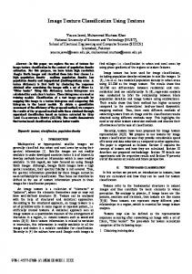
images, so color information is not currently used. Since we have made no attempt to normalize this variable space, many of these features may be interdependent and cannot be considered orthogonal. Furthermore, we make no claim that this feature set is complete in any way. In fact, it is expected that new types of features will be added, which will make this classification approach more accurate, more general or both. Figure 1 illustrates the construction of the feature vector by computing different groups of image features on the raw image and on the image transforms (Fourier, wavelet, Chebyshev) and transform combinations. As can be seen in the figure, not all features are computed for each image transform. For instance, object statistics are computed only on the original image, while Zernike polynomials are computed on the original image and its FFT transform, but not on the other transforms. Multiscale histograms, on the other hand, are computed for the raw image and all of its transforms. The permutations of feature algorithms and image transforms was selected intuitively to be a useful subset of the full set of permutations. Evaluation of this subset has established that this combinatorial approach yields additional valuable signals (see Figure 6). It is quite likely that further valuable signals could be obtained by calculating a more complete set of permutations.

transforms. In this work we also generated Chebyshev and wavelet transforms of the Fourier transform of the image. As will be described in Section 4, image content extracted from transforms of the image is a key contributor to the accuracy of the proposed image classifier. 2.2. Image features based on Chebyshev transform Chebyshev polynomials Tn (x) = cos(n·arccos(x)) (Gradshtein & Ryzhik, 1994) are widely used for approximation purposes. For any given smooth function, one can generate its Chebyshev approximant such as f (x) ' ΣN n=0 αn Tn (x), where Tn is a polynomial of degree n, and α is the expansion coefficient. Since Chebyshev polynomials are orthogonal (with a weight) (Gradshtein & Ryzhik, 1994), the expansion coefficients αn can be expressed via the scalar product αn = hf (x), Tn (x)i. For a given image I, its two-dimensional approximation through the Chebyshev polynomials is Iij = I(xi , yj ) ' ΣN n,m=0 αnm Tn (xi )Tm (yj ). The fast algorithm that was used in the transform computation takes two consequent 1D transforms, first for rows of the image, then for the columns of the resulting matrix, similarly to the implementation of 2D FFT. Chebyshev is used by the proposed image classifier both as a transform (with orders matching the image dimensions) and as a set of statistics. For the statistics, the maximum transform order does not exceed N = 20, so that the resulting coefficient vector has dimensions (1×400). The image features are the 32-bin histogram of the 400 coefficients. Since the Chebyshev features are computed on the raw image and on the Fourier-transformed image, the total number of image descriptors added to the feature vector is 64.

2.1. Basic image transforms Image features can be extracted not only from the raw image, but also from its transforms (Rodenacker & Bengtsson, 2003; Gurevich & Koryabkina, 2006; Orlov et al., 2006). Re-using feature extraction algorithms on image transforms leads to a large expansion of the feature space, with a corresponding increase in the variety of image content descriptors, but without a corresponding increase in algorithm complexity. For Fourier transform we used the FFTW (Frigo & Johnson, 2005) implementation of the Fourier transform. This transform results in complex-valued plane, of which only absolute values were used. For the wavelet transform, the standard MATLAB Wavelet toolbox functions were used to compute a Symlet 5, level 1 two-dimensional wavelet decomposition of the image. The Chebyshev transform was implemented by our group and is described in Section 2.2. Transform algorithms can also be chained together to produce compound

2.3. Image features based on Chebyshev-Fourier transform The Chebyshev-Fourier 2D transform is defined in polar coordinates, and uses two different kinds of orthogonal transforms for its two variables: distance and angle. The distance is approximated with Chebyshev polynomials, and the angle is deduced by Fourier harmonics, as described by Equation 1.

Ωnm (r, φ) = Tn ( 3

2r − 1)eimφ , 0 ≤ r ≤ R R

(1)

Fig. 1. The construction of the feature vector.

For the given image I, the transform is described by Equation 2.

the feature vector.

N

Iij ⇒ I(rk , φl ) '

N 2 X X

2.4. Image features based on Gabor wavelets βnm Ωnm (rk , φl ) (2)

n=0 m=− N 2

Gabor wavelets (Gabor, 1946) are used to construct spectral filters for segmentation or detection of certain image texture and periodicity characteristics. Gabor filters are based on Gabor wavelets, and the Gabor transform of an image I in frequency f is defined by Equation 3.

In the proposed image classifier, image descriptors are based on the coefficients βnm of the ChebyshevFourier transform, and absolute values of complex coefficients are used for image description (Orlov et al., 2006). The purpose of the descriptors based on Equation 2 is to capture low-frequency components (large-scale areas with smooth intensity transitions) of the image content. The highest order of polynomial used is N = 23, and the coefficient vector is then reduced by binning to 1×32 length. Since Chebyshev-Fourier features are computed on the raw image and on the Fourier-transformed image, this algorithm contributes 64 image descriptors to

Z

Z

GT (x, y, f ) =

(x−wx , y−wy )G(wx , wy , f )dwx dwy wx

wy

(3) where the kernel G(wx , wy , f ) takes the form of a convolution with a Gaussian harmonic function (Gregorescu, Petkov & Kruizinga, 2002), as described by Equation 5. 4

G(wx , wy ; f0 ) = e−

X 2 +γY 2 2α2

· ei(f0 X+φ)

2.6. Multi-scale histograms

(4)

X = wx cos(θ) + wy sin(θ)

This set of features computes histograms with varying numbers of bins (3, 5, 7, and 9), as proposed by (Hadjidementriou, Grossberg & Nayar, 2001). Each frequency range best corresponds to a different histogram, and thus variable binning allows measuring content in a large frequency range. The maximum number of counts is used to normalize the resulting feature vector, which has 1×24 elements. Multi-scale histograms are applied to the raw image, the Fourier-transformed image, the Chebyshevtransformed image, Wavelet-transformed image, and the Wavelet and Chebyshev transforms of the Fourier transform. Since each multi-scale histogram has 24 bins, the total number of feature elements is 6 × 24 = 144.

Y = −wx sin(θ) + wy cos(θ) The parameters of the transform are θ (rotation), γ (ellipticity), f0 (frequency), and α (bandwidth). As proposed by (Gregorescu, Petkov & Kruizinga, 2002), the parameter γ is set to 0.5, and α is set to 0.56 × 2π f0 . The Gabor features (GF) used in the proposed image classifier are defined as the area occupied by the Gabor-transformed image, as defined by Equation 5.

1 GF (f0 ) = GL

Z Z GT (x, y, f0 )dxdy. x

(5)

y

To minimize the frequency bias, these features are computed in a frequency range (f0 ∈ {fk }K k=1 ), and normalized with the low frequency component GL = GF (fL ). The frequency values that are used in the proposed image classifier are fL = 0.1 and f0 = [1, 2, ..., 7]. This results in 7 image descriptors, one for each frequency value that corresponds to high spectral frequencies, especially grid-like textures. Gabor filters are computed only for the raw image, and therefore 7 feature values are added to the feature vector.

2.7. Four-way oriented filters for first four moments For this set of features, the image is subdivided into a set of “stripes” in four different orientations (0o , 90o , +45o and -45o ). The first four moments (mean, variance, skewness, and kurtosis) are computed for each stripe and each set of stripes is sampled as a 3-bin histogram. Four moments in four directions with 3-bin histograms results in a 48element feature vector. Like the multi-scale histograms, the four moments are also computed for the raw image, the three transforms and the two compound transforms, resulting in 6 × 48 = 288 feature values.

2.5. Image features based on Radon transform The Radon transform (Lim, 1990) computes a projection of pixel intensities onto a radial line from the image center at a specified angle. The transform is typically used for extracting spatial information where pixels are correlated to a specific angle. In the proposed image classifier, the Radon features are computed by a series of Radon transforms for angles 0, 45, 90, and 135. Each of the resulting series values are then convolved into a 3-bin histogram, so that the resulting vector totals 12 entries. The Radon transform is computed for the raw image, the Chebyshev transform of the image, the Fourier transform of the image, and the Chebyshev transform of the Fourier transform. The Radon transform provides 12 feature values each time it is applied, so the total number of features contributed to the feature vector is 48.

2.8. Tamura features Three basic Tamura textural properties of an image are contrast, coarseness, and directionality (Tamura, Mori & Yamavaki, 1978). Coarseness measures the scale of the texture, contrast estimates the dynamic range of the pixel intensities, and directionality indicates whether the image favors a certain direction. For the image features we use the contrast, directionality, coarseness sum, and the 3bin coarseness histogram, totaling 6 feature values for this group. Tamura features are computed for the raw image and the 5 transforms (3 transforms plus 2 compound transforms), so that the total number of feature values contributed to the feature vector is 36. 5

2.9. Edge Statistics

computed only on the raw image and its Fourier transform. Therefore, the total number of feature values added by Zernike and Haralick features is 6 × 28 + 2 × 72 = 312.

Edge statistics are computed on the image’s Prewitt gradient (Prewitt, 1970), and include the mean, median, variance, and 8-bin histogram of both the magnitude and the direction components. Other edge features are the total number of edge pixels (normalized to the size of the image) and the direction homogeneity (Murphy et al., 2001), which is measured by the fraction of edge pixels that are in the first two bins of the direction histogram. Additionally, the edge direction difference is measured as the difference amongst direction histogram bins at a certain angle α and α + π, and is recorded in a four-bin histogram. Together, these contribute 28 values to the feature vector.

3. Feature Value Classification Due to the high dimensionality of the feature set, some of the features computed on a given image dataset are expected to represent noise. Therefore, selecting an informative feature sub-space by rejecting noisy features is a required step. In task-specific image classification, selection of relevant image features if often manual. For general image classification, however, feature selection (or dimensionality reduction) and weighting must be accomplished in an automated way. There are two different approaches of handling a large set of features; hard thresholding, in which a subset of the most informative features are selected from the pool of features, and soft thresholding, in which each feature is assigned a weight that corresponds to its informativeness. In the proposed classifier, we combine the two approaches by calculating weights for each feature, rejecting the least informative features, and using the remaining weighted features for classification. In the proposed implementation, the feature weight Wf of feature f is a simple Fisher Discriminant score (Bishop, 2006) described by Equation 6, PN (Tf − Tf,c )2 N · (6) Wf = c=1 PN 2 N −1 c=1 σf,c

2.10. Object Statistics Object statistics are calculated from a binary mask of the image resulting from applying a the Otsu global threshold (Otsu, 1979), and then finding all 8-connected objects in the resulting binary mask. Basic statistics about the segmented objects are then extracted, which include Euler Number (Gray, 1971) (the number of objects in the region minus the number of holes in those objects), and image centroids (x and y). Additionally, minimum, maximum, mean, median, variance, and a 10-bin histogram are calculated on both the objects areas and distances from objects centroids to the image centroid. These statistics are calculated only on the original image, and contribute 34 values to the feature vector.

where Wf is the Fisher Score, N is the total number of classes, Tf is the mean of the values of feature f in the entire dataset, Tf,c is the mean of the values of 2 feature f in the class c, and σf,c is the variance of feature f among all samples of class c. The Fisher Score can be conceptualized as the ratio of variance of class means from the pooled mean to the mean of withinclass variances. The multiplier factor of NN−1 is a consequence of this original meaning. All variances used in the equation are computed after the values of feature f are normalized to the interval [0, 1]. This weighting method was found to be simple, fast and effective for this classifier. After Fisher scores are assigned to the features, the weakest 35% of the features (with the lowest Fisher scores) are rejected. This number was selected empirically, based on our observations with several classification problems indicating that the classification accuracy reaches its

2.11. Zernike and Haralick features Zernike features (Teague, 1980) are the coefficients of the Zernike polynomial approximation of the image, and Haralick features (Haralick, Shanmugam & Dinstein, 1973) are statistics computed on the image’s co-occurrence matrix. While Zernike coefficients are complex-valued, absolute values are used as image descriptors. A detailed description of how these features are computed and used in the proposed classifier can be found at (Murphy et al., 2001). The number of values computed by Zernike and Haralick features are 72 and 28, respectively. While Haralick features are computed for the raw image and the 5 image transforms, Zernike features are 6

Accuracy (%)

peak when 45% of the strongest features are used. Since the accuracy is essentially unaffected in this wide range, we set the threshold in the middle of it. The resulting number of features used by this classifier is still significantly larger than most other image classifiers such as (Yavlinsky, Heesch & Ruger, 2006; Heller & Ghahramani, 2006; Rodenacker & Bengtsson, 2003), that use 120 to 240 different image content descriptors. These reduced and weighted features are used in a variation of nearest neighbor classification we named Weighted Neighbor Distances (WND-5). For feature vector x computed from a test image, the distance of the sample from a certain class c is measured by using Equation 7, P P|x| 2 2 p t∈Tc [ f =1 Wf (xf − tf ) ] (7) d(x, c) = |Tc | where T is the training set, Tc is the training set of class c, t is a feature vector from Tc , |x| is the length of the feature vector x, xf is the value of image feature f, Wf is the Fisher score of feature f, |Tc | is the number of training samples of class c, d(x, c) is the computed distance from a given sample x to class c, and p is the exponent, which is set to -5. That is, the distance between a feature vector and a certain class is the mean of all weighted distances (in the power of p) from that feature vector to any feature vector that belongs to that class. After the distances from sample x to all classes are computed, the class that has the shortest distance from the given sample is the classification result. While in simple Nearest Neighbor (Duda, Hart & Stork, 2000) only the closest (or k closest) training samples determine the class of the given test sample, WND-5 measures the weighted distances from the test sample to all training samples of each class, so that each sample in the training set can effect the classification result. The exponent (p) dampens the contribution of training samples that have a relatively large distance from the test sample. This value was determined empirically, and observations suggest that classification accuracy is not extremely sensitive to it. Figure 2 shows how the performance of several image classification problems (described in Section 4) respond to changes in the value of the exponent. As can be seen in the plot, a broad range of p between -20 and -4 gives comparable accuracies. This modification of the traditional NN approach provided us with the most accurate classification, compared to weighted NN (Duda, Hart & Stork, 2000) and Bayesian Networks with feature selec-

1

0.95

0.9

0.85

0.8

0.75

0.7 0.1

-P 0.5

1 ATT

10

5 Yale

Pollen

CHO

HeLa

Fig. 2. The effect of the exponent value −p on the accuracy of 5 image classification problems.

tion using greedy hill climbing (Kohavi & John, 1997). While the Bayesian network used a small set of image features (