Image Classification and Retrieval Using Elastic Shape Metrics Shantanu H. Joshi
Anuj Srivastava
Department of Electrical Engineering Florida State University Tallahassee, FL-32310
[email protected]
Department of Statistics Florida State University Tallahassee, FL-32306
[email protected]
Abstract— This paper presents a shape-based approach for automatic classification and retrieval of imaged objects. The shape-distance used in clustering is an intrinsic elastic metric on a nonlinear, infinite-dimensional shape space, obtained using geodesic lengths defined on the manifold. This analysis is landmark free, does not require embedding shapes in R2 , and uses ODEs for flows (as opposed to PDEs). Clustering is performed in a hierarchical fashion. At any level of the hierarchy, clusters are generated using a minimum dispersion criterion and a MCMC-type search algorithm is employed to ensure near-optimal configurations. The Hierarchical clustering potentially forms an efficient (O(log(n)) searches) tool for retrieval from large shape databases. Examples are presented for demonstrating these tools using shapes from the ETH-80 shape database. Keywords: shape clustering, shape classification, image
retrieval
I. I NTRODUCTION Unsupervised learning of visual object features is an important task in machine vision applications such as medical imaging, automatic surveillance, biometrics, and military target recognition. The imaged objects can be characterized in many ways: according to their colors, textures, shapes, movements, and locations. Of late, shape has been used as an important discriminant for identification and recognition of objects from images. Indeed, it is a desirable goal for an intelligent system to have automated tools for classifying and clustering objects according to the shapes of their boundaries. A. Past Shape-based Image Retrieval In general, there have been numerous approaches for including shapes in conjunction with color, intensity and textures for image indexing and retrieval. Many techniques, including Fourier descriptors [18], [17], Wavelet descriptors [20], chain codes, polygonal approximations [19], and moment descriptors [21] have been proposed and used in
various applications. Cortelazzo et al. [16] use chain codes for trademark image shape descriptions and string matching techniques. Jain and Vailaya [12] propose a representation scheme based on histograms of edge directions of shapes. A different approach by Mokhtarian et al. [14] uses curvature scale space methods for robust image retrieval from the Surrey fish dataset [13]. A majority of these methods have focused on the limited goal of fast shape matching and retrieval from large databases. Simple metrics using either Fourier or moment descriptors, or scale-space shape representations, may prove sufficient for retrieving shapes from a database. However they lack the tools and the framework for more advanced analysis, especially if one requires building probability models using the retrieved results. B. Past Shape Analysis Methods To address the above difficulties, and seek a a full statistical framework, Klassen, Srivastava et al. [2] adopt a geometric approach to parameterize curves by their arc lengths, and use their angle functions to represent and analyze shapes. Using the representations and metrics described in [2], Srivastava et al. [5] describe techniques for clustering, learning, and testing of planar shapes. One major limitation of this approach is that all curves are parameterized by arc length, and the resulting transformations from one shape into another are restricted to bending only. Local stretching or shrinking of shapes is not allowed. Mio and Srivastava [3] resolve this issue by introducing a representation that allows both bending and stretching of curves to compare and match shapes. It has been demonstrated in [3], that geodesics resulting from this approach seem more natural as interesting features, such as corners, are better preserved, thus leading to improved metrics in the shape space. We use the approach presented in [3] to represent and analyze shapes of closed curves. The basic idea is to represent
62
Fig. 1.
Example of a geodesic between a pair of shapes.
these curves as parameterized functions, not necessarily arc-length, with appropriate constraints, and define a nonlinear manifold C of closed curves. To remove similarity transformations, one forms a quotient space S = C/S, where S is the space of similarity transformations. Shapes of closed curves are analyzed as elements of S. The following section describes the shape representation scheme and briefly explains the construction of geodesics between any two given shapes on S. C. Elastic Shape Representation Scheme Let β be a parameterized curve of interest, of length l, and α = 2πβ/l be its re-scaled version. We will assume α : [0, 2π] → R2 to be a smooth, non-singular, orientationpreserving, parametric curve in the sense that α(s) ˙ 6= 0, ∀s ∈ [0, 2π]. Define the velocity vector of the curve as α(s) ˙ = eφ(s) ejθ(s) , where √ φ : [0, 2π] → R and θ : [0, 2π] → R are smooth, and j = −1. The function φ is the speed of α and measures the rate of stretching and compression, whereas θ is the angle made by α(s) ˙ with the X-axis and denotes bending. We will represent α via the pair ν ≡ (φ, θ), and denote by H the collection of all such pairs. In order to make the shape representation invariant to rigid motions and uniform scalings, we restrict shape representatives to pairs (φ, θ) satisfying the conditions; C = {(φ, θ) :
Z
2π 0
Z 2π 1 eφ(t) dt = 2π, θ(t)eφ(t) dt = π, 2π 0 Z 2π eφ(t) ejθ(t) dt = 0} ⊂ H, 0
where C is called the pre-shape space of planar elastic strings. Remark: Note that the pair (φ, θ) represents the shape of β, and thus ignores its placement, orientation, and scale. Shape deformations are studied using geodesics in the shape space S connecting them. Given two shapes ν1 and ν2 , computing a geodesic involves finding a tangent direction g ≡ (h, f ), such that the exponential map [1], expν1 (g) = ν2 . This is also represented by the geodesic flow Ψ1 (ν1 , g) = ν2 . Figure 1 shows such a geodesic between two shapes. Shape geodesics are computed under the following Riemannian metric [3]: Given (φ, θ) ∈ C, let hi and fi , i = 1, 2 be
tangent to C at (φ, θ). For a, b > 0, define Z 2π h(h1 , f1 ), (h2 , f2 )i(φ,θ) = a h1 (s)h2 (s) eφ(s) dt + 0 Z 2π b f1 (s)f2 (s) eφ(s) ds. 0
(1)
The parameters a and b control the tension and rigidity in the metric. The geodesic distance, (used as the shape metric) is now given by q d(ν1 , ν2 ) , k(h, f ))k(φ,θ) = h(h, f ), (h, f )i(φ,θ)
The remainder of the paper is organized as follows. Section II outlines a clustering algorithm using the geodesic lengths discussed above. The results and the performance of the clustering algorithm are demonstrated in Section III followed by the conclusion. II. S HAPE C LUSTERING Classical clustering algorithms on Euclidean spaces generally fall into two main categories: partitional and hierarchical [8]. Assuming that the desired number k of clusters is known, partitional algorithms typically seek to minimize a cost function Qk associated with a given partition of the data set into k clusters. Usually, the total variance of a clustering is a widely used cost function. Hierarchical algorithms, in turn, take a bottom-up approach. If the data set contains n points, the clustering process is initialized with n clusters, each consisting of a single point. The clusters are then merged successively according to some criterion until the number of clusters is reduced to k. Commonly used metrics include the distance of the means of the clusters, the minimum distance between elements of clusters, and the average distance between elements of the clusters. In this paper, we choose a value of k beforehand. A. Minimum-Variance Clustering Consider the problem of clustering n shapes (in S) into k clusters. To motivate our algorithm, we begin with a discussion of a classical clustering procedure for points in Euclidean spaces, which uses the minimization of the total variance of clusters as a clustering criterion. More precisely, consider a data set with n points {y1 , y2 , . . . , yn } with each yi ∈ Rd . If a collection C = {Ci , 1 ≤ i ≤ k} of subsets of Rd partitions the data into the total variance of Pkk clusters, P 2 C is defined by Q(C) = i=1 y∈Ci ky −µ P i k , where µ2i is the mean of data points in Ci . The term y∈Ci ky−µi k can be interpreted as the total variance of the cluster Ci . The total variance is used instead of the (average) variance to avoid placing a bias on large clusters, but when the data is fairly uniformly scattered, the difference is not
63
significant and either term can be used. The widely used kMeans Clustering Algorithm is based on a similar clustering criterion (see e.g. [8]). The soft k-Means Algorithm is a variant that uses ideas of simulated annealing to improve convergence [9], [7]. These ideas can be extended to shape clustering using d(ν, µi )2 instead of ky−µi k2 , where d(·, ·) is the geodesic length and µi is the Karcher mean [5] of a cluster Ci on the shape space. Clustering algorithms that involve finding means of clusters are only meaningful in metric spaces where means can be defined and computed. However, the calculation of Karcher means of large shape clusters is a computationally demanding operation. Therefore, it is desirable to replace quantities involving the calculation of means by approximations that can be derived directly from distances between the corresponding data points. Hence, we propose a variation that replaces d(ν, µi )2 with the average distancesquare Vi (ν) from ν to elements of Ci . If ni is the size P of Ci , then Vi (ν) = n1i ν 0 ∈Ci d(ν, ν 0 )2 . The cost Q associated with a partition C can be expressed as k X X X 2 d(νa , νb )2 . (2) Q(C) = n i i=1 νa ∈Ci b