Network Biology, 2016, 6(3): 55-64
Article
A node-similarity based algorithm for tree generation and evolution WenJun Zhang School of Life Sciences, Sun Yat-sen University, Guangzhou 510275, China; International Academy of Ecology and Environmental Sciences, Hong Kong E-mail:
[email protected],
[email protected] Received 6 August 2015; Accepted 28 September 2015; Published online 1 September 2016
Abstract In present study we proposed a node-similarity based algorithm for tree generation and evolution. In this algorithm, we assume that each isolated node is a node set at the beginning, two node sets with the greatest similarity tend to connect into a new node set firstly. Repeat this procedure, until all isolated nodes are combined into a tree. Pearson correlation measure, cosine measure, and (negative) Euclidean distance measure (the three measures are for interval attributes), contingency correlation measure (for nominal attributes), or Jaccard coefficient measure (for binary attributes) were used as the between-node similarity. In this way, all connections are sequentially generated and it thus forms the evolution process of a spanning tree of maximum likelihood. The similarity value of a connection can be considered as the weight of the connection. Matlab codes of the algorithm are provided. Keywords tree; generation; evolution; node similarity; algorithm.
Network Biology ISSN 22208879 URL: http://www.iaees.org/publications/journals/nb/onlineversion.asp RSS: http://www.iaees.org/publications/journals/nb/rss.xml Email:
[email protected] EditorinChief: WenJun Zhang Publisher: International Academy of Ecology and Environmental Sciences
1 Introduction Early in 1998, Watts and Strogatz developed a method for generating random graphs. Barabasi and Albert (1999) proposed a general mechanism for network evolution. Cancho and Sole (2001) algorithm can generate a variety of complex networks with diverse degree distributions. Fath et al. (2007) defined a step-by-step procedure for constructing an ecological network. Zhang (2011, 2012b, 2012c, 2012d, 2015a, 2016) proposed a series of methods and models for network generation and evolution. So far, research on network generation and evolution is still fewer. In present study, we will propose a node-similarity based algorithm for tree generation and evolution. Matlab codes of the algorithm are presented for further use. 2 Algorithm Suppose there are m isolated nodes (or objects, etc.) and n attributes. The raw data matrix is a=(aij)m×n. In the generation/evolution of a tree, I assume that in a set of isolated nodes (node sets), two nodes (node sets) with the greatest similarity tend to connect firstly. Pearson correlation measure, cosine measure, and (negative) IAEES
www.iaees.org
Network Biology, 2016, 6(3): 55-64
56
Euclidean distance measure (the three measures are for interval attributes), contingency correlation measure (for nominal (1, 2, 3…) attributes), or Jaccard coefficient measure (for binary (0, 1) attributes) can be used as the between-node similarity. Pearson correlation measure is (Zhang, 2011, 2016; Zhang et al., 2014; Zhang, 2012b, c; Zhang and Li, 2015) rij= ∑k=1n ((aik - aib)(ajk- ajb) )/(∑k=1n (aik - aib)2 ∑k=1n (ajk - ajb)2)1/2 i, j=1, 2,…,m where -1≤rij≤1, aib=∑k=1n aik/n, ajb=∑k=1n ajk/n, i, j=1, 2,…,m. Cosine measure is (Zhang, 2007; Zhang, 2012a) rij= ∑k=1n aik ajk/(∑k=1naik2 ∑k=1najk2)1/2 i, j=1, 2,…,m Euclidean distance measure is (Zhang, 2007, 2012a) dij= (∑k=1n (aik - ajk)2)1/2 Its negative value is used as the similarity measure rij= -dij Contingency correlation measure is (Zhang, 2007, 2012b; Zhang et al., 2014): rij=2(h/(s (p-1)))1/2-1
i, j=1, 2,…,m
where -1≤rij≤1, and h= s..(∑pi=1∑pj=1sij2/(si. s.j)-1) s.=∑pi=1 si. , si. =∑pj=1 sij , n.j =∑pi=1 sij where there are p available nominal values, i.e., t1, t2,…, tp, for attributes i and j, skl is the number of attributes of node i takes value tk and node j takes value tl, k, l= 1, 2, . . . , p. Jaccard coefficient measure is (Zhang, 2015b) rij=(e-(c+b))/(e+c+b)
i, j=1, 2,…,m
where -1≤rij≤1, c is the number of node pairs of 1 for attribute i but not for j; b is the number of node pairs of 1 for attribute j but not for i; e is the number of node pairs of 1 for both attribute i and attribute j. Between-node similarity matrix, r=(rij)m×m, is a symmetric matrix, i.e., r=r’. Calculate the similarity between node sets. Suppose there are two node sets, A and B. The similarity between A and B is defined as the greatest similarity between A and B
IAEES
www.iaees.org
Network Biology, 2016, 6(3): 55-64
rAB=max rij ,
57
i∈A, j∈B
At the start, m isolated nodes (or objects, etc.) are m node sets respectively. In all of node sets, choose two node sets with the maximal rAB to combine into a new node set, and the corresponding nodes, i and j, with the maximal rij, are connected. Repeat this procedure, until m isolated nodes are eventually combined into a tree. In this way, all connections are sequentially generated, and thus form the evolution process of a spanning tree (a more general network can be further generated from the spanning tree by adding more connections). The following are Matlab codes of the algorithm %Reference: Zhang WJ, Li X. 2016. A node-similarity based algorithm for tree generation and evolution. Selforganizology, 3(2): choice=input('Input a number to choose similarity measure (1: Pearson linear correlation; 2: Cosine measure; 3: (Negative) Euclidean distance; 4: Contingency correlation; 5: Jaccard coefficient): '); a=load(str); m=size(a,1); for i=1:m-1 for j=i+1:m ix=a(i,:); jx=a(j,:); if (choice==1) str='Pearson correlation'; ixbar=mean(ix); jxbar=mean(jx); aa=sum((ix-ixbar).*(jx-jxbar)); bb=sum((ix-ixbar).^2); cc=sum((jx-jxbar).^2); r(i,j)=aa/sqrt(bb*cc); end if (choice==2) str='Cosine measure'; aa=sum(ix.*jx); bb=sum(ix.^2); cc=sum(jx.^2); r(i,j)=aa/sqrt(bb*cc); end if (choice==3) str='(Negative) Euclidean distance'; r(i,j)=-sqrt(sum((ix-jx).^2)); end if (choice==4) str='Contingency correlation'; xx=[ix;jx]; pn=1; tt(1)=xx(1); for kk=1:max(size(xx)) jj=0; for ii=1:pn IAEES
www.iaees.org
58
Network Biology, 2016, 6(3): 55-64
if (xx(kk)~=tt(ii)) jj=jj+1; end; end if (jj==pn) pn=pn+1;tt(pn)=xx(kk); end; end for kk=1:pn for jj=1:pn temp(kk,jj)=0; for ii=1:max(size(ix)) if ((ix(ii)==tt(kk)) & (jx(ii)==tt(jj))) temp(kk,jj)=temp(kk,jj)+1; end; end end; end for kk=1:pn pp=0; for jj=1:pn pp=pp+temp(kk,jj); end ni(kk)=pp; end for kk=1:pn pp=0; for jj=1:pn pp=pp+temp(jj,kk); end nj(kk)=pp; end summ=0; for kk=1:pn summ=summ+ni(kk); end; xsquare=0; for kk=1:pn for jj=1:pn if (ni(kk)==0 | nj(jj)==0) continue; end xsquare=xsquare+temp(kk,jj)*temp(kk,jj)/(ni(kk)*nj(jj)); end; end xsquare=summ*(xsquare-1); r(i,j)=2*sqrt(xsquare/(summ*(pn-1)))-1; end if (choice==5) str='Jaccard coefficient'; bb=sum((ix==0) & (jx~=0)); cc=sum((ix~=0) & (jx==0)); dd=sum((ix~=0) & (jx~=0)); r(i,j)=(dd-(cc+bb))/(dd+cc+bb); end r(j,i)=r(i,j); end; end adj=zeros(m); r0=r; classid=1; IAEES
www.iaees.org
Network Biology, 2016, 6(3): 55-64
59
u(classid)=0; classnum(classid)=m; for i=1:classnum(classid) x(classid,i)=i; end tree=zeros(m); disp(['Step
Node
Node
' str]);
while (classnum(classid)>1) aa=-1e+10; for i=1:classnum(classid)-1 for j=i+1:classnum(classid) if (r(i,j)>aa) aa=r(i,j); end end; end aa1=0; for i=1:classnum(classid)-1 for j=i+1:classnum(classid) if (abs(r(i,j)-aa)temp) temp=r0(k,kk); end end; end; end; end; for k=1:m if (x(classid,k)==i) for kk=1:m if (x(classid,kk)==j) if (abs(r0(k,kk)-temp)r(i,j)) r(i,j)=r0(k,kk); end end; end; end; end; r(j,i)=r(i,j); end; end; end; fprintf('\nMatrix for tree evolution (elements are step IDs)') tree fprintf('\n') disp([str ' for each step']) corr=u(2:classid) fprintf('\nThe final adjacency matrix\n') adj
3 Application Example 3.1 Analysis of 54 human races and populations and 14 common HLA-DRB1 alleles Data of the world’s 54 human races and populations (nodes) and 14 common HLA-DRB1 alleles (attributes) are from Jia (2001) (Zhang and Qi, 2014; HLA_DRB1.txt; supplementary material). Here I use Pearson correlation measure to generate the tree. The process of tree evolution is listed in Table 1. The distribution of node degrees of final tree for 54 races and populations are indicated in Table 2, and the corresponding tree graph is drawn for convenient comparison using Java software (Zhang, 2012a), as indicated in Fig. 1.
IAEES
www.iaees.org
Network Biology, 2016, 6(3): 55-64
61
Table 1 The process of tree evolution of world’s 54 human races (nodes) and populations. Pearson Step
Node
Node
Pearson Step
Node
Node
corr.
Pearson Step
Node
Node
corr.
Pearson Step
Node
Node
corr.
corr.
1
24
28
0.9817
15
16
15
0.9182
29
39
32
0.8791
43
53
54
0.7374
2
33
35
0.9619
16
20
21
0.9182
30
49
13
0.8753
44
33
37
0.7330
3
28
26
0.9579
17
45
47
0.9181
31
11
10
0.8750
45
2
7
0.7211
4
5
11
0.9545
18
16
14
0.9144
32
44
43
0.8731
46
2
11
0.7065
5
42
44
0.9527
19
49
50
0.9141
33
10
31
0.8707
47
18
32
0.6789
6
45
46
0.9458
20
33
39
0.9136
34
46
48
0.8606
48
2
8
0.6581
7
49
51
0.9413
21
42
40
0.9103
35
5
4
0.8512
49
30
27
0.6562
8
36
40
0.9371
22
15
18
0.9092
36
18
19
0.8458
50
26
31
0.5708
9
33
34
0.9333
23
38
43
0.9082
37
5
1
0.8376
51
7
6
0.5526
10
16
17
0.9328
24
14
12
0.9077
38
1
3
0.8173
52
6
50
0.5353
11
49
52
0.9259
25
25
27
0.8962
39
3
9
0.8062
53
19
21
0.5132
12
46
42
0.9252
26
34
22
0.8915
40
22
23
0.8060
13
38
41
0.9199
27
12
11
0.8862
41
33
53
0.7828
14
28
25
0.9185
28
35
40
0.8823
42
29
30
0.7639
Node IDs from 1 to 54 represent Lahu-China, Dai-China, Yao-China, Guangdong Han-China, Dulong-China, Buyi-China, Thais, Yi-China, Hunan Han-China, Southern Han-China, Singapore Han-Singapore, Pumi-China, Shanghai Han-China, Liaoning Han-China, Shegyang Han-China, Northwest Han-China, Northern Han-China, Manchu-China, Japanese, Hokkaido-Japan, Uighur-China, Kazak-China, Siberian Nivkhs population, Siberian Udegeys population, Siberian Koryaks population, Siberian Eskimo, Siberian Chukchi population, South American Indians Ticuna, South American Indians Terena, Siberian Evenki population, Siberian Kets population, USA whites, Spanish, German, Romanians, Bulgarian, Greek, Polish, Turks, Macedonians, Israeli Arabs, Iranian Jews, Ashkenazi Jews-Germany, Libyan Jews, Moroccan Jews, Ethiopian Jews, Native population-Australia’s central desert, Yuendumu Native population-Australia, Kimberley native population-Australia, Cape York native population-Australia, North American blacks, and South African blacks.
Table 2 Node degrees for 54 races and populations. ID
1
2
3
4
5
6
7
8
9
Degree
2
3
2
1
3
2
2
1
1
10
11
12
13
14
15
16
17
18
ID Degree ID Degree ID Degree ID Degree ID Degree
IAEES
2
4
2
1
2
2
3
1
3
19
20
21
22
23
24
25
26
27
2
1
2
2
1
1
2
2
2
28
29
30
31
32
33
34
35
36
3
1
2
2
2
5
2
2
1
37
38
39
40
41
42
43
44
45
1
2
2
3
1
3
2
2
2
46
47
48
49
50
51
52
53
54
3
1
1
4
2
1
1
2
1
www.iaees.org
Network Biology, 2016, 6(3): 55-64
62
Fig. 1 The generated tree of 54 races and populations. Node IDs are explained in Table 1.
3.2 Analysis of 12 Chinese human populations and 17 HLA-DQB1 alleles Data of the 12 Chinese human populations (nodes) and 17 common HLA-DQB1 alleles (attributes) (1217; HLA_DQB1.txt; supplementary material) are from Geng et al. (1995), Chang et al. (1997), Mizuki et al. (1997, 1998), et al. Use Pearson cosine measure and results to generate the tree. The process of tree evolution is as follows Step 1 2 3 4 5 6 7 8 9 10 11
Node 7 6 6 10 10 4 11 3 7 6 8
Node 8 10 4 5 7 3 12 2 1 11 9
Cosine measure 0.9764 0.97057 0.94927 0.94407 0.93692 0.92891 0.92311 0.90887 0.85977 0.78742 0.75927
where the node IDs from 1 to 12 represent Tibetan, Uighur, Kazak, Xingjiang Han, Taiwanese, Hong Kong,
IAEES
www.iaees.org
Network Biology, 2016, 6(3): 55-64
63
Northern Han, Shanghai Han, Hunan Han, Manchu, Buyi, and Dai. The corresponding tree is indicated in Fig. 2.
Fig. 2 The generated tree of 12 Chinese populations. Node IDs are explained in text.
4 Discussion The present algorithm is based on similarity between nodes. The node sets with greater similarity tend to connect than that with less similarity. The final tree achieved is thus a spanning tree with maximum likelihood. The similarity value of a connection can be considered as the weight of the connection. Considering the generality of such mechanism of tree generation in nature, it is expected to be a general method for tree generation. This algorithm can produce connections sequentially, thus can reflect the process of tree evolution. Further studies or applications on the algorithm are expected in the future.
Acknowledgment We are thankful to the support of High-Quality Textbook Network Biology Project for Engineering of Teaching Quality and Teaching Reform of Undergraduate Universities of Guangdong Province (2015.6-2018.6), from Department of Education of Guangdong Province, Discovery and Crucial Node Analysis of Important Biological and Social Networks (2015.6-2020.6), from Yangling Institute of Modern Agricultural Standardization, and Project on Undergraduate Teaching Reform (2015.7-2017.7), from Sun Yat-sen University, China.
References Barabasi AL, Albert R. 1999. Emergence of scaling in random networks. Science, 286(5439): 509 Cancho RF, Sole RV. 2001. Optimization in complex networks. Santafe Institute, USA Chang YW, Hawkins BR. 1997. HLA Class I and Class II frequencies of a Hong Kong Chinese population based on bone marrow donor registry data. Human Immunology, 56: 125-135 Geng L, Imanishi T, Tokunaga K, et al. 1995. Determination of HLA class II alleles by genotyping in a
IAEES
www.iaees.org
64
Network Biology, 2016, 6(3): 55-64
Manchu population in the northern part of China and its relationship with Han and Japanese populations. Tissue Antigens, 46:111-116 Fath BD, Scharler UM, Ulanowiczd RE, Hannone B. 2007. Ecological network analysis: network construction. Ecological Modeling, 208: 49–55 Jia ZJ. 2001. Polymorphism of HLA-DRB1 gene in southern Chinese populations. PhD Thesis. 46-47, Sun Yat-sen University, Guangzhou, China Mizuki N, Ohno S, Ando H et al. 1998. Major histocompatibility complex class II alleles in an Uygur population in the Silk Route of Northwest China. Tissue Antigens, 51: 287-292 Mizuki N, Ohno S, Sato T et al. 1997. Major histocompatibility complex class II alleles in Kazak and Han populations in the Silk Route of Northwest China. Tissue Antigens, 50: 527-534 Watts D, Strogatz S. 1998. Collective dynamics of ’small world’ networks. Nature, 393:440-442 Zhang WJ. 2007. Computer inference of network of ecological interactions from sampling data. Environmental Monitoring and Assessment, 124: 253-261 Zhang WJ. 2011. Constructing ecological interaction networks by correlation analysis: hints from community sampling. Network Biology, 1(2): 81-98 Zhang WJ. 2012a. A Java software for drawing graphs. Network Biology, 2(1): 38-44 Zhang WJ. 2012b. Computational Ecology: Graphs, Networks and Agent-based Modeling. World Scientific, Singapore Zhang WJ. 2012c. How to construct the statistic network? An association network of herbaceous plants constructed from field sampling. Network Biology, 2(2): 57-68 Zhang WJ. 2012d. Modeling community succession and assembly: A novel method for network evolution. Network Biology, 2(2): 69-78 Zhang WJ, 2015a. A generalized network evolution model and self-organization theory on community assembly. Selforganizology, 2(3): 55-64 Zhang WJ. 2015b. Calculation and statistic test of partial correlation of general correlation measures. Selforganizology, 2(4): 55-67 Zhang WJ. 2016. Selforganizology: The Science of Self-Organization. World Scientific, Singapore Zhang WJ, Li X. 2015. Linear correlation analysis in finding interactions: Half of predicted interactions are undeterministic and one-third of candidate direct interactions are missed. Selforganizology, 2(3): 39-45 Zhang WJ, Qi YH. 2014. Pattern classification of HLA-DRB1 alleles, human races and populations: Application of self-organizing competitive neural network. Selforganizology, 1(3-4): 138-142 Zhang WJ, Qi YH, Zhang ZG. 2014. Two-dimensional ordered cluster analysis of component groups in self-organization. Selforganizology, 1(2): 62-77
IAEES
www.iaees.org