Mar 26, 1976 - Hence, the higher resolution visual appearance of the spectrum of. Fig. l(a) over that of the spectrum of Fig. l(b) is due to .the transformation f(x) ...
Pa( w ) =
(4)
fHKF
where K is the M X M forward-backward estimate of the autocorrelation matrix obtained by including only the principal eigenvectors (toeffect noise reduction) and setting the corresponding principal eigenvalues equal to one. Hence P
K
yv;."
= i-I
For our example (Fig. l(b)) p = 2 and M = 12. It is clear then that the MUSIC algorithm has higher resolution than the Fourier-based spectrum estimator.
relates to the ability of a spectrum estimator to determine whether one or two sinusoidal components, closely spaced in frequency, is present in white noise. Then, the problem of assessing the resolutionofa spectrum estimator is naturally addressed within the framework of statistical hypothesis testing. One could, for example, determine the probabilityof detecting the two sinusoids when they are present versus the probabilityof deciding there are two sinusoids whenonlyone sinusoid is present,i.e., the probability of false alarm [7]. In summary, it is hoped that this example will serve to illustrate a spectrum thedifficulties arising in assessing theresolutionof estimator by solely visual means. REFERENCES
11.
RELATING SPECTRUM OF FIG. l(a) TO
SPECTRUM
OF
FIG. l(b)
We now show that the spectrum estimators given by (3) and (4) are related. Since M
yv;"
I= i-1
M
D
where I is the identity matrix, one can rewrite (3) as
-
R. Schmidt, "Multiple emitter location and signal parameter estimation," in Proc. RADC SpectralEstimation Workshop, pp. 243-258, Rome, NY, 1979. A. Nuttall, "Spectral analysis of a univariate process with bad data points, via maximumentropy,andlinearpredictivetechniques," NUSC Tech. Rep. TR 5303,New London, C r , Mar. 26,1976. T.T. Ulrych and R. W. Clayton, "Time series modeling andmaximum entropy," Phys. Earth Planetary Interiors, vol. 12, pp. 188-200, Aug. 1976. W. 5. Liggett, "Passive sonar: Fitting models to multiple time series," in SignalProcessing, J. W. R. Criffiths et a/., Eds. NewYork: Academic Press, 1973. N. L. Owsley, "A recent trend in adaptivespatialprocessingfor sensor arrays: Constrained adaptation," in Signal Processing, J. W. R. Criffiths et dl., Eds. New York: Academic Press, 1973. D. H.Johnson, "The application of spectral estimation methods to bearing estimation problems," Proc. I € € € , vol. 70, no. 9, pp. 1018-1028, Sept. 1982. Personal communication with D. W. Tufts.
1
1-
EHkf
A Reduced Structure of the Frequency-Domain Block LMS Adaptive Digital Filter
Note that since D
JAE CHON LEE AND CHONG KWAN UN i-I
In this letter, it is shown that the frequency-domain block LMS (FBLMS) adaptive digital filter (ADF) for the block length of one reduces to thefrequencrdomain LMS (FLMS) ADF. Using the relation between the two convergence factors of the FBLMS and FLMS ADFs, it is possible to predict the steadystateperformance of the former from that of the latter.
M
D
i-I
i-1 M
i- 1
=
€HE=
INTRODUCTION
1
we have that
0
< P a ( w ) < 1.
(6)
Hence, the higher resolution visual appearance of the spectrum of Fig. l(a) over thatof the spectrum of Fig. l(b) is due to .the transformation f ( x ) = 1/(1 - x ) over the region 0 < x < 1. It is clear also then that since the transformation is monotonic with x the peaks of the spectrum of Fig. l(b), which are not plainly visible, are identical to the sharppeaks of the spectrum of Fig. l(a). For frequency estimationin whichone estimates the frequencies by the peaks of the spectrum the two spectrum estimators will produce identical results. Similar observations have been made in [6]. Ill. DISCUSSION
The example discussedraisesseveral important points. Firstly, visual inspection of spectrais not a scientifically valid means of assessing resolution of a spectrum estimator. In fact the "resolution" of the MUSIC algorithmcould be improved by defininganew spectrum estimator
as an example. Secondly,andmost importantly, one must first determine what resolution is. Assume, for example, that resolution
Recently, there has been considerable interest among researchers in efficient realization of an adaptive digital filter (ADF) using the block least mean-square (BLMS) algorithms [I], [2]. In the BLMS ADFs, the filter weightsare updated once in every block rather than at every sampling instant. The BLMS ADF can be realized efficiently in the frequency domain using the fast Fourier transform (FFT). The frequency-domain BLMS (FBLMS) ADFconvergesfast even when theinput signal is highly correlated [I]. However, despite these excellent advantages, the steady-state performance of the FBLMS ADF has not been analyzed yet. In this letter, we investigate the relation between the FBLMS ADF and the frequency-domain L M S (FLMS) ADF that is operated on the sample-by-sample basis, and discuss the use of the result in studying the steady-state performance of the FBLMS ADF. THE FBLMS ADAPTIVE DIGITALFILTER As a performance criterion in adjusting the weights, the block mean-squared error (BMSE) may be formulated. Then, using the method of steepest descent, one can have a time-domain or a frequency-domain B L M S algorithm. One realization structure of the FBLMS ADF using FFT and the overlap-save sectioning procedure is Manuscript received April 27, 1984. The authors are with the Department of Electrical Engineering, Korea Advanced Institute of Science and Technology, Seoul, Korea.
KIl8-9219/84/12~-1816M.W@I984 IEEE
1816
PROCEEDINGS
OF THE IEEE, VOL. 72, NO
12. DECEMBER 1984
INPUT
Xn
Fig. 1. Realization of a n FBLMS A D F using FFT and overlap-save sectioning procedure ( N = L M - 1 + N,and N, > 0). [Note: S/P = serial-to-parallel conversion and P/S parallel-to-serial conversion.]
+
-
Fig. 2.
Realization of an FBLMS ADF for block length of one
shown i n Fig. 1 [I], [2]. In this figure, M , L , and N are the number of the weights, the block length, and the transform length, respectively. The adjustment algorithm for the frequency-domain weights { vk,i > of the filter in the kth blockis given as [I]
Then, using { vn,i ) from (2), we obtain the filter output y, as N-1 Yn
=
N-1 Sn,;vn,;
i-0
1;
- exp { j Z q ( N - 1 ) i / ~ ) ]=
c
sn,;wn,, (3)
i-0
where where the overbar denotes complex conjugate, and s k , , and f k , , are the i t h frequency components of the FFTs of the a!gmented Input and error signals, respectively [see Fig. 11. In (I), a / f k , iis a convergence factor, a and f k , ;being aconstant and the estimated value of the frequency-domain power E[s,,;Z,, ;], respectively. REDUCED STRUCTURE F O R BLOCK LENGTH OF ONE
For the case of the block length beingequal to one, the structure of Fig. 1 becomes that of Fig. 2 when N, = 0. Unlike in Fig. 1, the sectioning procedure required just after adjusting the weights is not necessary in Fig. 2 since N = M . Note that the arithmetic operations in Fig. 2 replace the inverse FFT operation for computing the filter output, the FFT operation for updating the weights, and the sectioning procedure shown i n Fig. 1. Using the variables shown in Fig. 2 and assuming %,; = 0 for all I, an alternative algorithm for weight adjustment is obtained as follows. First, the weights { v n + , , ; ) are represented as n
vn+l,i=
(a/im,;)Sm,,fm,;=exp{-j2n(N-l)i/N} m-0 n
.
( u / i m , , ) s m , , e m , O G ; G N-I. m-0
PROCEEDINGS O F THE IEEE. VOL. 72, N O 12, DECEMBER 1%
(2)
n-1
wn,i'
1
(4)
~ ( ~ / i m , i ) ~ r n , , e m . m=O
Assuming w0,;= 0 for all i, we have from (5) the following weight adjustment algorithm: 1 w ~ + ~ = ,wn,i , + x(a/in,,)Sn,,en, 0
G iG N
- 1.
(5)
A structure for the ADF represented by (3) and (5) is shown in Fig. 3. It i s seen that, unlike in Fig. 1, one inverse FFT and one FFT operations have been cancelled out for the block length of one. It is interesting to note that the structure of Fig. 3 is the same as that of the F L M S ADF proposed by Narayan et a/. [3]. Thus when the convergence factor of the F L M S ADFis given as y / f , , , , wehave from (5) the following relation between a and y : a = Ny.
(6)
Therefore, using (6), one can predict the steady-state behavior of the F B L M S ADF in terms of that of the F L M S ADF. Our results of computer simulation indicate that given the values of y and M , the steady-state performances of the FBLMS ADFs with a satisfying (6) are almost the sameregardless of L . (For L = 1, the convergence behaviors of the FBLMS and F L M S ADFs were identical.)
1817
INPUT
xn
-%,o
+ u.
-Yn
DESIRD RESWNSE
dn
Fig. 3.
A reduced structure of the FBLMS ADF for block length of one.
Recently, we have analyzed the performance of the FLMS ADF [4]. According to our study, the value of y can be chosen such that the steady-state performance of the FLMS ADF satisfies the design specification. Consequently, the value of a for the FBLMS ADF can be chosen i n the sameway using (6). Since the general convergence behaviors of the FBLMS and FLMS ADFs appear to be similar, one can also take the same approach as used for the case of the FLMS ADF in analyzing the performance of the FBLMS ADF. This aspect is under study. REFERENCES
[ l ] D. Mansourand A. H. Gray, Jr., “Unconstrained frequency-domain adaptivefilter,” /€€E Trans. Acoust., Speech, SignalProcess., vol. ASSP-30, pp. 726-734, Oct. 1982. [2] G. A.Clark, S. R. Parker,and S. K . Mitra, “A unified approach to time- andfrequency-domainrealizationof FIR adaptive digital filters,” / € € E Trans. Acousf., Speech, Signal Process., vol. ASSP-31, pp. 1073-1083, Oct.1983. [3] S. S. Narayan, A. M. Peterson, and M. J. Narasimha,“Transform domain L M S algorithm,” /€€E Trans. ACOUS~., Speech, Signal Process., vol. ASSP-31, pp. 609-615, June 1983. [4] J. C. Lee and C. K. Un, “Performanceoftransform-domain LMS adaptive digital filters,”submitted for publication in /E€€ Trans. Acousf., Speech, Signal Process.
weighting, signals arriving in timesequence areamplitude-weighted to produce low sidelobes in the frequency domain. A significant measure of the performance of a weighting functionin suppressing leakage i s the highest sidelobe level (relative to the main lobe). Figures have been published [ I ] of the highest sidelobe level for a wide variety of weighting functions. However, there seems to be no indication that for some of the weighting functions, the sidelobe levels are sensitive to the value of N , the number of data samples. In particular, it has been found that for weighting functions that rest on a platform (discontinuity at the boundary), the published figures apply only when N is reasonably large (more than 50-100 samples). Examples of weighting functions on a platformare the Hamming and the Blackman-Harris functions. When the number of samples is small, as in the case of pulse Doppler radar where 16 or 32 samples are commonly used, the sidelobe levels of weighting functions on a platform are significantly higher than the published figures. For the weighting functions that taper smoothly to zero at the boundaries, such as the Hann and Blackman functions, the sidelobe levels are not sensitive to the values of N. In this letter the discrete Fourier transform (DFT) is derived in a particular form for temporal weightings [2] defined by K
w(n) =
a,cos(Zakn/N),
for0
< n < N - 1.
k-0
Sidelobe levels of Weighting Functions with a Platform when the Numberof Samples ( N ) is Small F. E. CHURCHILL The highest sidelobe level is a figure of merit of weighting functions. It has been found that published figures [I] for weightinn functions that rest on a platform, e.g, Hamming, BlackmanHarris, apply only when N is .large. The sdelobe levels are significantly higher than the published figures when N is small.
The formofthe expressionreveals that the sidelobe levelsare bounded from below by the platform height w(0). The expression for the DFT is used to calculate the approximate sidelobe levels, for values of N from 16 to approaching an infinite number, for two weighting functions with a platform, the Hamming and the Blackman-Harris, and for two weighting functions with a zero platform, theHannandthe Blackman.The sidelobe sensitivity to N for weighting functions with a platform is thereby demonstrated. 11.
SPECTRAL
WINDOW O F TIME-WEIGHTINGFUNCTION
The Hamming and Blackman-Harris (three-term) time-weighting functions are defined for the DFT by
w ( n )= a. - a, cos ( 2 n n / N )
+ a2 cos( 4 n n / N ) ,
n = 0 , 1 , 2 ; . . , ( N - I )( .1 ) I.
INTRODUCTION
Weightings are used in either the frequency or time domains, i n signal processing, to reduce spectral leakage. Computation may be easier in one domain than in the other. In the case of temporal
The ak coefficients are
a0
dl Manuscript received April 22, 1983; revised December 28, 1983. The author is with the Systems Engineering Department, Tactical Ground Defense Systems, Raytheon Company, Missile Systems Division, Bedford, M A 01730, USA.
a2
Blackman-Harris (-61 dB)
0.54 0.46 0
0.44959 0.49364 0.05677
The spectral window is found by performing a DFT on w(n), a set of time samples. The DFT of w ( n ) is
0018-9219/84/1200-1818901.00
1818
Hamming
a1984 IEEE
PROCEEDINGS O F THE IEEE. VOL. 72, NO 12, DECEMBER 1984