Automated mound detection using lidar and object-based image analysis in Beaufort County, South Carolina* Dylan S. Davis,1 Matthew C. Sanger,1 and Carl P. Lipo1 1
Department of Anthropology, Binghamton University, Binghamton, New York, USA
Corresponding author: Dylan S. Davis;
[email protected]; Department of Anthropology, Binghamton University, 4400 Vestal Parkway E., Binghamton, NY 13902, USA ABSTRACT The study of precontact anthropogenic mounded features—earthen mounds, shell heaps, and shell rings—in the American Southeast is stymied by the spotty distribution of systematic surveys across the region. Many extant, yet unidentified, archaeological mound features continue to evade detection due to the heavily forested canopies that occupy large areas of the region, making pedestrian surveys difficult and preventing aerial observation. Object-based image analysis (OBIA) is a tool for analyzing light and radar (lidar) data and offers an inexpensive opportunity to address this challenge. Using publicly available lidar data from Beaufort County, South Carolina, and an OBIA approach that incorporates morphometric classification and statistical template matching, we systematically identify over 160 previously undetected mound features. This result improves our overall knowledge of settlement patterns by providing systematic knowledge about past landscapes. KEYWORDS Lidar; South Carolina; remote sensing; object-based image analysis (OBIA); semi-automatic survey The study of topographically distinct anthropogenic features—shell rings, middens, shell heaps, and earthen mounds—has been a primary focus of Southeastern archaeology since its inception (e.g., Anderson 2004; Claflin 1931; Crusoe and DePratter 1976; Marquardt 2010; Moore 1894a, 1894b; Putnam 1875; Squier and Davis 1848; Swallow 1858; Trinkley 1985). The shape, configuration, and distribution of these distinctive cultural features are routinely used as the basis for studies of demographic change, environmental alteration, social organization, and site formation in the Americas (Brennan 1977; Carr and Sears 1985; Claassen 1986; Crusoe and DePratter 1976; Lightfoot and Cerrato 1989; Peacock et al. 2005; Reitz 1988; Russo 2004; Trinkley 1985). Yet, while mounds are key components to our understanding of the archaeological past, the lack of systematic survey of large areas hinders our knowledge of their numbers and spatial patterns. In particular, wherever vegetation is dense—as is common across much of the American Southeast—we have an inconsistent and partial knowledge of these archaeological features. Today, substantial effort is placed on archaeological investigations that utilize noninvasive and nondestructive remote sensing techniques. These approaches offer opportunities to expand our ability to incorporate systematic methods to archaeological surveying across large *
This is an Accepted Manuscript of an article published by Taylor & Francis in Southeastern Archaeology on June 21, 2018, available online: http://www.tandfonline.com/10.1080/0734578X.2018.1482186.
1
areas (e.g., Custer et al. 1986; De Laet et al. 2007; Doneus et al. 2014; Eskew 2008; Freeland et al. 2016; Kirk et al. 2016; Krasinski et al. 2016; Kvamme 2013; Lasaponara et al. 2014; Riley 2009; Schneider et al. 2015; Thompson et al. 2011; Traviglia and Torsello 2017; Trier et al. 2015; Van Ess et al. 2006). These approaches utilize sensors, such as cameras on aerial platforms, to acquire landscape level information about the archaeological record. These sensors measure visible light or other ranges of electromagnetic spectra. While using aerial sensors in archaeology is certainly not new (e.g., Capper 1907; Engelbach 1929; Lindbergh 1929a, 1929b), the use of photos has largely been rooted in manual analysis where the analyst must visually seek out features of interest. This approach, while productive, limits the ability of remote sensing to be useful in large areas. Additionally, it leads to inconsistent evaluation of materials, makes repeated evaluation costly, and restricts the approach to imagery easily evaluated in an intuitive fashion (e.g., visible light photography). One promising alternative to manual evaluation of remote sensing data for detecting features of interest is the use of object-based image analysis (OBIA) (Blaschke 2010; Freeland et al. 2016). While growing in popularity across the natural sciences (e.g., Freeland et al. 2016; Magnini et al. 2016; Riley 2009; Schneider et al. 2015; Trier et al. 2015), remote sensing applications have remained largely unexplored in Southeastern archaeology. The potential for using OBIA to explore remote sensing data is particularly great for the identification and location of two forms of topographic anomalies with precontact origins: earthen constructions (i.e., mounds) and shell constructions (i.e., mounds and rings). The archaeological record of the American Southeast once had thousands of these mound features, and their study provides much of the basis of our knowledge about the prehistory of the region. Unfortunately, urban development over the last 50 years has led to the widespread destruction of many shell rings and earthen mounds (Stalter et al. 1999:864). In Beaufort County, South Carolina, for example, less than 5% of the surface has been well surveyed according to the state archaeological site files. Much of the area is under dense vegetation, making systematic surface survey difficult, if not impossible. At the same time, the rate of land development for golf courses and residential complexes has increased substantially over the last 30 years, along with a doubling of Beaufort’s population (US Census 2010). Sea level projections estimate that up to 30,000 acres of dry land in the Beaufort County area will be submerged by 2040, including nearly total inundation of many coastal islands (National Oceanic and Atmospheric Administration [NOAA] 2015). As loss of the archaeological record continues, it is urgent that we implement efforts to systematically investigate the remaining landscape, and to do so with the greatest detail, coverage, and the lowest cost possible. Consequently, remote sensing innovations have tremendous potential to address this challenge. In this paper, we explore an approach to implement a systematic remote sensing method to identify artificial mounded features using Beaufort County, South Carolina, as a case study (Figure 1).
2
Figure 1. The study area of Beaufort County, South Carolina. Mounds and their challenges Identifying topographic features such as precontact anthropogenic mounds and rings is complicated by their morphological diversity in terms of outline, profile, and size (see Russo 2006; also see Riley 2009); these can be circular, oval, rectangular, or have irregular and effigy outlines. Even within a single set of features, such as rings, there can be variation. Within South Carolina and Georgia, for example, features identified as “shell rings” have circular or “Cshaped” outlines, whereas in Florida, shell rings are often “U-shaped” and far more amorphous (Russo 2006:24). Mounded features have a variety of two-dimensional elevation profiles ranging from rectangular to triangular to trapezoidal or, in the case of rings, bimodal. Additionally, size also varies: shell rings in South Carolina and Georgia are substantially smaller than those in Florida. If one is searching for rings in Florida, any automatic detection algorithm must account for objects that can occupy spaces of 250 m2 or greater, whereas in South Carolina, these features are unlikely to exceed 150 m2 (see Russo 2006). Fortunately, much of the variability in mound morphology is stylistic (sensu Dunnell 3
1978) and thus, regionally specific. Therefore, algorithms designed to detect these features can be trained using regionally specific information that examines the number of potential dimensions of variability. Using regional samples to train algorithms provides a statistical basis for defining parameters. It is important to note, however, that parameters are contingent on sampling; to be useful in new areas, algorithms must be trained to set appropriate parameters for those study regions. One additional challenge for identifying mounds and shell rings comes from the fact that anthropogenic topographic features resembling earthworks may in fact be relatively recent phenomena. Among such examples are remnants of levee constructions, modern construction projects, and golf courses. Golf courses, in particular, often have shape and topographic characteristics that closely resemble mounds. Minimizing false positives caused by modern land disturbance requires additional information to be utilized, such as surrounding land use or ecological context. Ultimately, isolating features that are recent in origin often requires subsurface sampling or comparisons with historic data. Lidar One excellent source for topographic information on the scale of landscapes come from light and radar (lidar) instruments.1 Lidar data are produced using an active remote sensing system that emits electromagnetic energy in the form of light and records the return times of these pulses to calculate distance. By measuring the time-of-flight of many different light pulses simultaneously, lidar data are unique in their ability to reflect ground surfaces, even in densely vegetated areas (Jensen 2007). The recent set of lidar-based studies to explore the archaeological record, including the recent discovery of several hundred new Mayan archaeological sites in Guatemala, provide excellent examples for how lidar can reveal previously hidden landscapes (Clynes 2018; Inomata et al. 2018; see also Chase et al. 2014; Evans et al. 2013; Johnson and Oiumet 2018; Weishampel et al. 2011; Witharana et al. 2018). Within the Southeast, lidar has primarily been used to produce high-resolution maps of known mound sites (e.g., Thompson et al. 2016; Wood and Pluckhahn 2017) but has not been utilized for prospection of new archaeological deposits. In the context of the mounds and rings of the Southeast, lidar is particularly significant, as these features are often now covered by dense forests, making their detection difficult with traditional pedestrian surveys (e.g., Nance 1983; Schiffer et al. 1978) or impossible with aerial photography. Lidar data are represented in three dimensions as “point clouds” in which each measurement has a spatial coordinate in three-dimensional space. The most common files for storing lidar points are LAS format (or LAZ for compressed versions). LAS files store collections of lidar points in a binary format which provides efficient storage of large amounts of lidar data (Samberg 2007). LAS files include data on the geographic position for each mapped point plus information about collection methods, minimum and maximum values, and classification values. Often the raw LAS files are converted into Digital Elevation Models (DEMs) in which the raw data are processed and interpolated into a regular grid of elevation points. The use of DEMs for analysis typically reduces the detail that would be available in the raw lidar data but also ensures regular topographic coverage for regions of interest. For our analyses, we used DEM files generated by NOAA (2013) from the raw LAS files. The DEMs are interpolations of “bare ground” lidar returns from the original data using nearest neighbor and inverse distance weighting (IDW) algorithms to create elevation values every 1.2 m. We conducted all subsequent analyses using our algorithm for mound detection on this raster dataset. 4
For archaeological purposes, lidar data are usually filtered to limit analysis to those points representing bare ground elevations. In areas with obscured topographies, such as forests or vegetated landscapes, however, not all light pulses will penetrate to the ground surface. Isolating the bare ground data requires selecting those points that come from the pulses of light that are the last to return to the sensor as opposed to earlier returned pulses that are reflected off of intervening vegetation. The penetration of lidar signals through vegetation can vary and is dependent upon the power of the lidar transmitter, the wavelength of light used in the pulse, the scanning angle of the sensor, the density of the vegetation, and the type of vegetative cover present in an area (Clark et al. 2004; Crow et al. 2007). In areas for which lidar data are missing due to heavy vegetation, interpolation algorithms must be used to estimate the values of locations that lack data (Li and Heap 2014). Given any particular lidar dataset, one must devise algorithms that can isolate spatial patterns of topography of interest. These algorithms search through the data and identify matches of points that meet criteria on overall shape, size, local relief, and degree of symmetry. The challenge to the archaeologist is to find the most effective set of criteria that can best identify features of interest with the fewest false positives and false negatives. Often it is useful to include data from other sources including vegetation, distance to other features, land-use classification, and so on. Lidar data have a number of limitations for the detection of cultural features. The spacing of ground sampling generated through the process of lidar scanning is a major factor in the quality of the data for use in identifying features. If lidar data are too sparse with point spacings that are too far apart, the dataset will have a low spatial resolution and thus may not be adequate for recognizing distinct topographic features, especially those that are small (Johnson and Ouimet 2014). The coverage of lidar over surfaces is also impacted by the degree to which the emitted light was able to penetrate vegetation. In densely forested areas, for example, the intensity of survey must be sufficient to ensure adequate returns from beneath the canopy (Bater and Coops 2009). The utility of lidar data given the degree of coverage also depends on the complexity of the terrain: the more complexity that one wishes to explore, the more coverage is required. In the same way, features that have low topographic profiles will require greater degree of coverage and increased precision in the spatial positions. Finally, the utility of data will also be impacted by the raw data that are resampled to produce DEMs (Bater and Coops 2009). Analytic approaches to remote sensing data There are two primary means to analyze remote sensing data: pixel-based and object-based methods (Sevara et al. 2016). Pixel-based approaches rely on spectral values encoded in raster data. Using a library of known values associated with targets of interest, it is possible to divide raster images into a series of classes that represent those targets. In contrast, OBIA methods identify features using a number of morphological characteristics, including the spectral difference within image objects, object shape, and neighborhood analysis (Blaschke 2010:3). By incorporating multiple morphological parameters, OBIA is well suited for identifying spatially discrete features that are small, spectrally diverse, and/or structurally similar. In the case of mound detection—where features vary primarily in terms of topographic structure (e.g., shape, circularity, and elevation profiles; Larsen et al. 2017)—lidar data analyzed through OBIA shows great promise. More specifically, mound detection algorithms can take advantage of multiresolution segmentation and template matching (Cerrillo-Cuenca 2017; Magnini et al. 2016; Schneider et 5
al. 2015; Trier et al. 2015). Segmentation involves the splitting of an image into individual components based on brightness thresholds, elevation profiles, shape, and texture (Haralick et al. 1973; Mao and Jain 1992). The process isolates individual pixels and then systematically expands sets of pixels to larger units. For each step, the algorithm segments the units based on differences in texture, color, and shape, which results in the division of an image into representations of surface features. For example, mounded features display sudden changes in topography which are divided in the segmentation process. Circular features on the ground are represented by circular image objects of the same shape and size of the mound on the ground (e.g., Freeland et al. 2016; Jahjah et al. 2007; Magnini et al. 2016; Sevara et al. 2016; Van Ess et al. 2006). Multiresolution segmentation is a method that uses iteration to combine attributes about texture, shape, compactness, and color into the segmentation procedure, thereby increasing its accuracy compared to other image segmentation methods (Burt et al. 1981; Mao and Jing 1992; Silberberg et al. 1980). Template-matching is an additional OBIA approach for isolating features of interest. Template-matching involves iteratively searching images using a constructed framework and evaluating statistical similarity (Trier and Pilø 2012; Trier and Zortea 2012; Trier et al. 2008; Trier et al. 2015). However, the approach can produce significant false positives, as the templates simply produce portions of the image that are most similar to the specified morphology of the template. For mounds, false positives often occur as recent cultural features caused by construction along roadsides, stream banks, dams, golf courses, residual buildings, and farming (Riley 2009:82). To minimize false positives, one can use land-use maps and roadway shapefiles to filter out features that are best explained as the result of recent activity unrelated to prehistory. Materials and methods Beaufort County, South Carolina, contains a large number of recognized archaeological sites, a significant number of which are earthen or shell mounds (Frierson 2002; Stephenson 1971). Shell rings are the earliest unambiguous evidence of sedentary or near-sedentary occupations of the coastal portions of the county (Russo 2006; Trinkley 1980). These deposits offer information about the subsistence and settlement patterns of Archaic period hunter-gatherer groups living along the coast. Later Woodland period deposits include earthen mounds (Trinkley 1989), a form that becomes increasingly common over time, particularly during the later Mississippian period (Anderson 1989). Much of Beaufort County consists of forests and heavily vegetated marshland. These conditions make traditional pedestrian surveys (e.g., Michie 1980) difficult. Thus, much of our knowledge about the archaeological record is limited to portions where land has been cleared for development or for which pedestrian access is relatively easy. Consequently, our knowledge of settlement patterns is limited to more inland regions. Fortunately, in 2008 and 2009, the National Oceanic and Atmospheric Administration generated lidar data of many of the counties along the coast in South Carolina. While generated to provide information about coastal flooding, these datasets offer archaeologists a means of studying these landscapes that are otherwise hidden by dense vegetation. Currently available NOAA (2017) data are Digital Elevation Models (DEMs) with a spatial resolution of 1.2 m. These DEMs are derived from the original raw lidar data using nearest neighbor and inverse distance weighted (IDW) interpolation algorithms. These data offer topographic elevation values for every 1.2 m, a resolution that is generally sufficient for identifying mound-scale archaeological features on the order of tens of meters (see Beck et al. 6
2007).2 As such, a majority of known mounded features (including shell rings) in South Carolina are large enough to be identified at this resolution. The data, however, are unlikely to be able to detect small mounds that are just a couple of meters in diameter. Thus, the smallest mounds will be systematically missing from the results of this study. In addition to the horizontal spatial resolution, the vertical precision of the lidar data is 15 cm, meaning that for a mound to be detectable it must rise at least 15 cm from the ground surface. One issue that faces the analyst is excluding cultural features with discrete topographic expressions that are not part of the archaeological record. Contemporary features related to recent development (e.g., golf courses, housing developments, roadways, construction piles) often have shapes that are similar to prehistoric mounds. In order to minimize false positives from these features, we used United States Geological Survey (USGS) land-use maps and road maps from the South Carolina Department of Transportation. These maps provided us examples of features (n = 393) that we used to create negative templates for topographically distinct nonmound features (e.g., roadways, waterbodies, linear features, and building imprints). Pre-processing steps Using DEM data downloaded from NOAA, we created four different rasters that highlight topography in different ways: slope, maximum focal statistics, red-relief image map (RRIM), and range focal statistics. Each of these rasters became the source information used for our analytic techniques of feature extraction. Slope. Slope rasters highlight elevation changes on a landscape (Figure 2) and emphasize sinks and rises on ground surfaces such as mounds (Larsen et al. 2017; Podobnikar 2012; Prufer et al. 2015; Riley 2009; Thompson and Prufer 2015). Maximum focal statistics. Maximum focal statistic rasters are calculated by evaluating each data point and conducting a nearest neighbor analysis of elevation values where the maximum elevations are identified over a moving window (Podobnikar 2012). The produced raster exaggerates topographic features in the landscape and allows for smaller objects to be seen more easily (Figure 2). Hillshade. Hillshade rasters are a type of shaded-relief map that highlights elevation changes in a landscape (Figure 2). One of the drawbacks to this raster type is that the source of the light in the model causes distortion that can obscure certain landscape features (Devereux et al. 2008). For this reason, we also use a shade-free relief map known as a red-relief image map. RRIM. Red-relief image mapping produces rasters that are based on the concept of topographic openness (Chiba et al. 2008; Yokoyama et al. 2002). Using System for Automated Geoscientific Analyses or SAGA (Conrad et al. 2015), an open-source GIS platform, we calculated topographic openness. For our DEM data we calculated an “openness parameter” (I) for each point following Equation 1 (Chiba et al. 2008:1073). 𝐼 =
𝑂𝑝 − 𝑂𝑛 2
Equation 1
In Equation 1, Op is an assessment of positive openness—which calculates topographic concavity—and On is an assessment of negative openness—which calculates topographic 7
convexity. We used SAGA to calculate topographic openness. RRIM is created by overlapping I with a slope gradient in ArcGIS. We then used the RRIM values to create a colored map that shows slope in a red gradient and I as a white-to-black gradient. RRIM conversions of raw data highlights relatively slight landscape features in lidar data regardless of viewing angle (Ichita et al. 2016; Inomata et al. 2017).
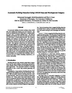
Figure 2. Comparison map of DEM processing approaches: (a) DEM; (b) maximum focal statistics; (c) slope; (d) RRIM; (e) hillshade. The focal statistic raster emphasizes the outline of the shell ring when compared to the regular DEM. Slope clearly reveals the border of ring and mound structures present on the landscape. RRIM provides a clearer and less distorted view of topographic changes than hillshade and picks up on smaller features in addition to the larger shell ring present in the image. Range focal statistics. Rasters constructed from range focal statistics show overall elevation changes in a DEM within a specific neighborhood. Because mounds are characterized by sudden changes in elevation relative to the local topography, range focal statistics can indicate locations with steep changes thus areas that might have mound features. An algorithm for topographic feature identification Our algorithm for identifying mounds follows the process illustrated in Figure 3. We conducted our template matching procedure using eCognition (Trimble 2016). To account for 8
morphological variability in mound shape, we created 15 templates using a series of 29 mound features (Figure 4), of which 6 are known archaeological mounds and the remainder were manually identified in lidar data (Lipo et al. 2018). Our use of 15 templates to identify mounded features enables us to assess the degree to which our template choice influences the features that are identified. The product of the template matching consists of two correlation-coefficient maps that represent the fit to our positive and negative templates. These provide statistical probabilities on a scale from -1 to 1 (where -1 is extremely unlikely and 1 is a definitive match) of mound locations for the study area.
Figure 3. The feature identification algorithm processing steps. We also conducted multiresolution segmentations of each raster image using area and circularity as classificatory parameters. In this process, we assess each of the areas matching the templates by their sizes and shapes (Freeland et al. 2016) as well as asymmetry and compactness. Asymmetry characterization helps to eliminate natural phenomena while compactness characterization tends to be associated with artificial rather than natural features (Kvamme 2013:55).
9
Figure 4. Locations of all sample features used in the positive template creation process. We minimized false positives from our list of identified features through a number of steps in ArcGIS (ESRI 2017; Table 1). First, we used the elevation range raster to identify only those features that exhibit a total positive elevation difference of greater than or equal to 0.5 m but less than 5.0 m. This range is consistent with most mounds and rings known in the Beaufort County area (see Russo 2006), but it excludes all features that are topographically less than 0.5 m in relative elevation. Thus, mounds that have been flattened, eroded, bulldozed, or which have low relief will be systematically missing from our results. While the vertical resolution of the raw lidar data (15 cm) suggest that lower profile features can potentially be identified, the inclusion of small elevation differences results in an excessive number of false positives. Small differences due to natural processes—such as levee banks, tree fall, and animal burrows—would potentially appear as features with less than 0.5 m of elevation difference. As such, we decided to limit our search to those features we were more certain that we could identify as prehistoric mounds in this area. Table 1. Classification Parameters Used in Multiresolution Segmentation. Parameter Threshold 10
Area Circularity Asymmetry Compactness
0–120 pixels (0–150 m2) ≥ 0.6 0–0.3 ≥ 1.0
Note: Parameters are based on the ranges known from mounds previously identified in the Beaufort County study area. Circularity is measured on a scale from 0 to 1 with 1 being a perfect circle. Asymmetry and compactness are also unitless ratios, with the higher the number representing greater levels of asymmetry or compactness. Second, we used a land-use map to isolate mound features that were located on or within 5 m of land classified as developed or disturbed by the USGS. These locations are often associated with false positive results due to their association with recent activity (Riley 2009). For the same reason, we excluded all results that fell within 10 m of roadways and 20 m of major highways. Third, we removed all features with topographic profiles that have slopes less than five degrees and greater than 50 degrees. We chose this range based on our ground surveys of 22 mound features in the study region (also see Wood and Johnson 1978). Fourth, we used the template matching process to reduce our results to the most statistically viable: we excluded those results with a 75% likelihood of identification for negative templates. Fifth, we created a new raster by subtracting the negative correlation coefficient from the positive correlation coefficient. We rejected results that fell in areas of this raster with negative values. Sixth, we used the RRIM raster to visually inspect the remaining objects and remove those that could be identified as historic or recent. Results Our initial identification process produced 7,115 potential features. After inspecting these results using the steps above, we obtained 186 results that are likely to represent cultural mound features, of which 15 appear the most promising (Table 2). We chose the features we deemed to be the “most likely” to be archaeological mounds based on the visual inspection of each result using a combination of the DEM, slope raster, and RRIM, as these three datasets provide the necessary elevation information and visualization capabilities to view identified features. Paying particular attention to the features’ immediate surroundings (i.e., are they located in a highly developed or undeveloped area?), elevation profile, size, and shape, the 15 high-likelihood features exhibited elevation profiles and morphological properties consistent with known mounds and were located in entirely undeveloped regions. The medium- and low-likelihood features exhibited morphological characteristics that were noticeably different than known mounds and/or had relative locations that contained greater levels of modern development and disturbance. Table 2. Manual Processing Result Likelihoods. Likelihood Mound Ring Total Low 55 21 76 Medium 64 31 95 High 9 6 15 Total 128 58 186
11
In October 2017, we conducted a ground survey to assess a sample of five identified features (representing a 33% sample of high-likelihood objects; Figure 5). This number represents features that were accessible on public land and without the use of a boat.
Figure 5. Locations of surveyed sites: (a) all sites visited during ground truth survey; (b) newly identified shell ring; (c) newly identified earthen mound. The locations of (b) and (c) are indicated in map (a). Three of the five features that we evaluated in our ground evaluation are mounds that were previously identified (see Supplemental Table 1 for all site numbers associated with identified features). Two of the features, however, are new discoveries (not yet recorded as archaeological sites). These two new mound features have evaded detection despite decades of 12
traditional survey (e.g., Michie 1980; Russo 2006; Russo and Heide 2001; Stalter et al. 1999). The first of these is a precontact shell ring with a ~15-m-wide plaza and a ~1.5-m-high arc (Figure 5). The second newly identified site is a precontact mound that rises approximately 2 m from the surrounding area and shows evidence of previous looting (Figure 5). While the ultimate determination of our method’s efficacy requires a larger sample size and further ground survey, our results are promising. Many of the 186 identified sites in Beaufort County are previously unrecorded mounds, and our future work will focus on documenting each of these identified locations (Figure 6). Only 20 of the features identified here appear in the South Carolina Archaeological Site Files, indicating that the majority of topographic anomalies identified here are not recorded as archaeological sites (see Supplemental Table 1). As such, our method has the potential to unveil over 160 new archaeological sites in the Beaufort County area.
Figure 6. Geographic locations of all 186 features identified by our algorithm. Conclusions Overall, our study demonstrates how semi-automatic object-based image analysis using lidar 13
data can provide a significant source of information about precontact landscapes in heavily vegetated areas. As Nance (1983) points out, the use of traditional pedestrian survey approaches in heavily vegetated areas is problematic, and in many instances, the results of such surveys are inadequate (also see Schiffer et al. 1978). Lidar offers a cost-effective means to economically identify features in areas that would otherwise be expensive to study. While successful, our method excludes potential mounds that have been plowed or otherwise disturbed by modern or natural phenomena. As such, mounds and rings that are potentially in the most need of active protection—namely, those that are being eroded, leveled by development, or otherwise reduced in size—are less likely to be identified using the specific parameters implemented here. New datasets with increased vertical and horizontal spatial resolution plus the inclusion of additional parameter potentially offer a means of identifying these smaller—and often overlooked—archaeological deposits. Our algorithm also relies partially on a comprehensive template that contains records of various known mound morphologies. As such, if a mound feature varies too far from the mounds in our template they are also unlikely to be identified. This shortcoming is resolvable by ground testing our results and continuing to apply our algorithm to other locations. As we confirm more features, they can be added to our template, making it more robust and more accurate. Despite these limitations, our algorithm enabled us to identify topographic features for an entire county of 2,481 km2 in the span of one week. This same venture in terms of traditional pedestrian survey would be measured in years (see Nance 1983). Importantly, this method is adaptable to other locations. As we gathered results from our pedestrian evaluations, we were able to update our templates to include newly discovered features and to add false positives to our negative templates. Our preliminary examination of data from Charleston County, South Carolina, produced about 1,000 potential features. The use of OBIA offers promise in identifying previously undocumented archaeological features. This knowledge will help more fully document Native American settlement patterns and land use prior to European contact. With the discovery of a new potential shell ring, the roughly 50 currently known shell rings in the American Southeast (Russo 2006:40) are likely to represent only a sample of extant features. Through the use of remote sensing data and OBIA approaches we can be more confident about our knowledge of these important classes of mound features and can better contribute to the protection of these important deposits. Notes 1. Contrary to common thought, lidar is not an acronym for “light detection and ranging” but is merely a blend of the terms “light” and “radar” (see Goyer and Watson 1963). 2. Beck and colleagues (2007) conducted tests on satellite imagery data to assess the visualization capabilities of different spatial resolutions. Although different from lidar-derived DEM datasets, the implications of spatial resolution on the suitability of remote sensing data for archaeological prospection remains the same: better spatial resolution allows for the detection of smaller objects and greater numbers of archaeological deposits. Acknowledgments The authors would like to thank the anonymous peer reviewers for their constructive comments on the manuscript. We also wish to thank Katherine Seeber for her help in conducting ground surveys. The authors are responsible for any errors.
14
Data availability statement All related datasets are available through Binghamton University’s Open Repository (Lipo et al. 2018). Disclosure statement No potential conflict of interest was reported by the authors. Funding Funding was provided by National Geographic award number HJ-107R-17 and Binghamton University. Notes on the contributors Dylan S. Davis is a graduate student at Binghamton University and focuses his research on human-environmental interactions and remote sensing applications for archaeological analysis. His geographic focus lies in coastal and island regions, including the American Southeast. Matthew C. Sanger is the Director of the Public Archaeology program and Assistant Professor of Anthropology at Binghamton University. His research includes Native American occupation of the southeast coastline, including South Carolina, Georgia, and Florida. Carl P. Lipo is a Professor of Anthropology at Binghamton University. His research focus centers on the use of remote sensing approaches as a means for studying the archaeological record. His work includes studies in Eastern North America and Oceania. ORCID Dylan S. Davis https://orcid.org/0000-0002-5783-3578 Matthew C. Sanger http://orcid.org/0000-0002-0553-8809 Carl P. Lipo https://orcid.org/0000-0003-4391-3590 References Cited Anderson, David G. 1989 The Mississippian in South Carolina. In Studies in South Carolina Archaeology: Essays in Honor of Robert L. Stephenson, edited by Albert C. Goodyear and Glen T. Hanson, pp. 101–132. Anthropological Studies 9, Occasional Papers of the South Carolina Institute of Archaeology and Anthropology. University of South Carolina, Columbia. Anderson, David G. 2004 Archaic Mounds and the Archaeology of Southeastern Tribal Societies. In Signs of Power: The Rise of Cultural Complexity in the Southeast, edited by Jon L. Gibson and Philip J. Carr, pp. 270–299. University of Alabama Press, Tuscaloosa. Bater, Christopher W., and Nicholas C. Coops 2009 Evaluating Error Associated with Lidar-derived DEM Interpolation. Computers & Geosciences 35(2):289–300. Beck, Anthony, Graham Philip, Maamoun Abdulkarim, and Daniel Donoghue 2007 Evaluation of Corona and Ikonos High Resolution Satellite Imagery for Archaeological
15
Prospection in Western Syria. Antiquity 81(311):161–175. Blaschke, Thomas 2010 Object-Based Image Analysis for Remote Sensing. ISPRS Journal of Photogrammetry and Remote Sensing 65(1):2–16. Brennan, Louis A. 1977 The Midden Is the Message. Archaeology of Eastern North America 5:122–137. Burt, Peter J., Tsai-Hong Hong, and Azriel Rosenfeld 1981 Segmentation and Estimation of Image Region Properties through Cooperative Hierarchical Computation. IEEE Transactions on Systems, Man, and Cybernetics 11(12):802–809. Capper, John E. 1907 Photographs of Stonehenge as seen from a War Balloon. Archaeologia 60:571. Carr, Christopher, and Derek W. G. Sears 1985 Toward an Analysis of the Exchange of Meteoritic Iron in the Middle Woodland. Southeastern Archaeology 4(2):79–92. Cerrillo-Cuenca, Enrique 2017 An Approach to the Automatic Surveying of Prehistoric Barrows through LiDAR. Quaternary International 435:135–145. Chase, Arlen F., Diane Z. Chase, Jaime J. Awe, John F. Weishampel, Gyles Iannone, Holley Moyes, Jason Yaeger, and M. Kathryn Brown 2014 The Use of LiDAR in Understanding the Ancient Maya Landscape. Advances in Archaeological Practice 2(3):208–221. Chiba, Tatsuro, Shin-ichi Kaneta, and Yusuke Suzuki 2008 Red Relief Image Map: New Visualization Method for Three-Dimensional Data. International Archives of the Photogrammetry, Remote Sensing and Spatial Information Sciences 37(B2):1071–1076. Claassen, Cheryl 1986 Shellfishing Seasons in the Prehistoric Southeastern United States. American Antiquity 51(1):21– 37. Claflin, William H. 1931 The Stalling’s Island Mound, Columbia County, Georgia. Papers of the Peabody Museum of American Archaeology and Ethnology, Volume XIV, No. 1. Harvard University, Cambridge, Massachusetts. Clark, Matthew L., David B. Clark, and Dar A. Roberts 2004 Small-Footprint Lidar Estimation of Sub-canopy Elevation and Tree Height in a Tropical Rain Forest Landscape. Remote Sensing of Environment 91(1):68–89. Clynes, Tom 2018 Exclusive: Laser Scans Reveal Maya “Megalopolis” Below Guatemalan Jungle. National Geographic. National Geographic Society, February 1. Electronic Document, https://news.nationalgeographic.com/2018/02/maya-laser-lidar-guatemala-pacunam/, accessed February 3, 2018.
16
Conrad, Olaf, Benjamin Bechtel, Michael Bock, Helge Dietrich, Elke Fischer, Lars Gerlitz, Jan Wehberg, Volker Wichmann, and Jürgen. Böhner 2015 System for Automated Geoscientific Analyses (SAGA) v. 2.1.4. Geoscientific Model Development 8(7):1991–2007. Crow, Peter, Sue Benham, Bernard Devereux, and Gabriel Amable 2007 Woodland Vegetation and Its Implications for Archaeological Survey Using LiDAR. Forestry 80(3):241–252. Crusoe, Donald L., and Chester B. DePratter 1976 New Look at the Georgia Coastal Shell Mound Archaic. Florida Anthropologist 29(1):1–23. Custer, Jay F., Timothy Eveleigh, Vytautas Klemas, and Ian Wells 1986 Application of Landsat Data and Synoptic Remote Sensing to Predictive Models for Prehistoric Archaeological Sites: An Example from the Delaware Coastal Plain. American Antiquity 51(3):572–588. De Laet, Véronique, Etienne Paulissen, and Marc Waelkens 2007 Methods for the Extraction of Archaeological Features from Very High-Resolution Ikonos-2 Remote Sensing Imagery, Hisar (Southwest Turkey). Journal of Archaeological Science 34(5):830–841. Devereux, Bernard J., Gabriel S. Amable, and Peter Crow 2008 Visualisation of LiDAR Terrain Models for Archaeological Feature Detection. Antiquity 82(316):470–479. Doneus, Michael, Geert Verhoeven, Clement Atzberger, Michael Wess, and Michal Ruš 2014 New Ways to Extract Archaeological Information from Hyperspectral Pixels. Journal of Archaeological Science 52:84–96. Dunnell, Robert C. 1978 Style and Function: A Fundamental Dichotomy. American Antiquity 43(2):192. Engelbach, Reginald 1929 The Aeroplane and Egyptian Archaeology. Antiquity 3(12):47–73. Eskew, Katherine 2008 Using LiDAR and GIS to Detect Prehistoric Earthworks in the Yazoo Basin, Mississippi. MA thesis, Department of Anthropology, California State University, Long Beach. ESRI 2017
ArcGIS Version 10.5. Environmental Systems Research Institute, Inc., Redlands, California.
Evans, Damian H., Roland J. Fletcher, Christophe Pottier, Jean-Baptiste Chevance, Dominique Soutif, Boun Suy Tan, Sokrithy Im, Darith Ea, Tina Tin, Samnang Kim, Christopher Cromarty, Stéphane De Greef, Kasper Hanus, Pierre Bâty, Robert Kuszinger, Ichita Shimoda, and Glenn Boornazian 2013 Uncovering Archaeological Landscapes at Angkor Using LiDAR. Proceedings of the National Academy of Sciences 110(31):12595–12600. Freeland, Travis, Brandon Heung, David V. Burley, Geoffrey Clark, and Anders Knudby 2016 Automated Feature Extraction for Prospection and Analysis of Monumental Earthworks from Aerial LiDAR in the Kingdom of Tonga. Journal of Archaeological Science 69:64–74.
17
Frierson, John L. 2002 South Carolina Prehistoric Earthen Indian Mounds. Master’s thesis, Department of History, University of South Carolina, Columbia. Goyer, Guy G., and Robert D. Watson 1963 The Laser and Its Application to Meteorology. Bulletin of the American Meteorological Society 44(9):564–575. Haralick, Robert M., Karthikeyan Shanmugam, and Its ’hak Dinstein 1973 Textural Features for Image Classification. IEEE Transactions on Systems, Man, and Cybernetics SMC-3(6):610–621. Ichita, Shimoda, Haraguchi Tsuyoshi, Chiba Tatsuro, and Shimoda Mariko 2016 The Advanced Hydraulic City Structure of the Royal City of Angkor Thom and Vicinity Revealed through a High-Resolution Red Relief Image Map. Archaeological Discovery 4(1):22–36. Inomata, Takeshi, Flory Pinzón, José Luis Ranchos, Tsuyoshi Haraguchi, Hiroo Nasu, Juan Carlos Fernandez-Diaz, Kazuo Aoyama, and Hitoshi Yonenobu 2017 Archaeological Application of Airborne LiDAR with Object-Based Vegetation Classification and Visualization Techniques at the Lowland Maya Site of Ceibal, Guatemala. Remote Sensing 9(6):563. Inomata, Takeshi, Daniela Triadan, Flory Pinzón, Melissa Burham, José Luis Ranchos, Kazuo Aoyama, and Tsuyoshi Haraguchi 2018 Archaeological Application of Airborne LiDAR to Examine Social Changes in the Ceibal Region of the Maya Lowlands, edited by John P. Hart. PLOS ONE 13(2):e0191619. Jahjah, Munzer, Carlo Ulivieri, Antonio Invernizzi, and Roberto Parapetti 2007 Archaeological Remote Sensing Application Pre-Post War Situation of Babylon Archaeological Site—Iraq. Acta Astronautica 61(1–6):121–130. Jensen, John R. 2007 Remote Sensing of the Environment: An Earth Resource Perspective. 2nd ed. Pearson Prentice Hall, Upper Saddle River, New Jersey. Johnson, Katharine M., and William B. Ouimet 2018 An Observational and Theoretical Framework for Interpreting the Landscape Palimpsest through Airborne LiDAR. Applied Geography 91:32–44. Johnson, Katharine M., and William B. Ouimet 2014 Rediscovering the Lost Archaeological Landscape of Southern New England Using Airborne Light Detection and Ranging (LiDAR). Journal of Archaeological Science 43:9–20. Kirk, Scott Detrich, Amy E. Thompson, and Christopher D. Lippitt 2016 Predictive Modeling for Site Detection Using Remotely Sensed Phenological Data. Advances in Archaeological Practice 4(1):87–101. Krasinski, Kathryn E., Brian T. Wygal, Joanna Wells, Richard L. Martin, and Fran Seager-Boss 2016 Detecting Late Holocene Cultural Landscape Modifications Using LiDAR Imagery in the Boreal Forest, Susitna Valley, Southcentral Alaska. Journal of Field Archaeology 41(3):255–270.
18
Kvamme, Kenneth 2013 An Examination of Automated Archaeological Feature Recognition in Remotely Sensed Imagery. In Computational Approaches to Archaeological Spaces, pp. 53–68. Left Coast Press, Walnut Creek, California. Larsen, Bernie P., Simon J. Holdaway, Patricia C. Fanning, Tim Mackrell, and Justin I. Shiner 2017 Shape as an Outcome of Formation History: Terrestrial Laser Scanning of Shell Mounds from Far North Queensland, Australia. Quaternary International 427:5–12. Lasaponara, Rosa, Giovanni Leucci, Nicola Masini, and Raffaele Persico 2014 Investigating Archaeological Looting Using Satellite Images and GEORADAR: The Experience in Lambayeque in North Peru. Journal of Archaeological Science 42:216–230. Li, Jin, and Andrew D. Heap 2014 Spatial Interpolation Methods Applied in the Environmental Sciences: A Review. Environmental Modelling & Software 53:173–189. Lightfoot, Kent G., and Robert M. Cerrato 1989 Regional Patterns of Clam Harvesting Along the Atlantic Coast of North America. Archaeology of Eastern North America 17:31–46. Lindbergh, Charles A. 1929a Colonel and Mrs. Lindbergh Aid Archaeologists. Carnegie Institute Reports. Carnegie Institute, New York. Lindbergh, Charles A. 1929b The Discovery of the Ruined Maya Cities. Science 70:12–13. Lipo, Carl P., Matt Sanger, and Dylan Davis 2018 Automated Mound Detection using LiDAR and Object-Based Image Analysis in Beaufort County, SC. Anthropology Datasets 3. Binghamton University Open Repository. Electronic document, https://orb.binghamton.edu/anthro_data/3, accessed March 15, 2018. Magnini, Luigi, Cinzia Bettineschi, and Armando De Guio 2016 Object-Based Shell Craters Classification from LiDAR-Derived Sky-View Factor. Archaeological Prospection 24(3):211–223. Mao, Jianchang, and Anil K. Jain 1992 Texture Classification and Segmentation Using Multiresolution Simultaneous Autoregressive Models. Pattern Recognition 25(2):173–188. Marquardt, William H. 2010 Shell Mounds in the Southeast: Middens, Monuments, Temple Mounds, Rings, or Works? American Antiquity 75(3):551–570. Michie, James L. 1980 An Intensive Shoreline Survey of Archeological Sites in Port Royal Sound and the Broad River Estuary, Beaufort County, South Carolina. Research Manuscript Series 167. Institute of Archaeology and Anthropology, University of South Carolina, Columbia. Moore, Clarence Bloomfield
19
1894a Certain Sand Mounds of the St. John’s River, Florida, Part I. Journal of Academy of Natural Sciences of Philadelphia 10(1):1–103. Moore, Clarence Bloomfield 1894b Certain Sand Mounds of the St. John’s River, Florida, Part II. Journal of Academy of Natural Sciences of Philadelphia 10(2):129–246. Nance, Jack D. 1983 Regional Sampling in Archaeological Survey: The Statistical Perspective. Advances in Archaeological Method and Theory 6:289–356. National Oceanic and Atmospheric Administration 2013 2013 SC DNR Lidar: Beaufort County Point Cloud files with Orthometric Vertical Datum North American Vertical Datum of 1988 (NAVD88) using GEOID12B. Electronic document, https://coast.noaa.gov/htdata/lidar1_z/geoid12b/data/5104/, accessed February 8, 2017. National Oceanic and Atmospheric Administration 2015 Sea Level Rise Adaptation Report Beaufort County, South Carolina. Electronic document, http://www.scseagrant.org/pdf_files/Beaufort-Co-SLR-Adaptation-Report-Digital.pdf, accessed February 12, 2018. National Oceanic and Atmospheric Administration 2017 Coastal Topographic LiDAR. Electronic document, https://coast.noaa.gov/digitalcoast/data/coastallidar, accessed March 4, 2018. Peacock, Evan, Janet Rafferty, and S. Homes Hogue 2005 Land Snails, Artifacts and Faunal Remains: Understanding Site Formation Processes at Prehistoric/Protohistoric Sites in the Southeastern United States. In Archaeomalacology: Molluscs in Former Environments of Human Behavior, edited by Daniella Bar-Yosef, pp. 6–17. Oxbow Books, Oxford. Podobnikar, Tomaž 2012 Detecting Mountain Peaks and Delineating Their Shapes Using Digital Elevation Models, Remote Sensing and Geographic Information Systems Using Autometric Methodological Procedures. Remote Sensing 4:784–809. Prufer, Keith M., Amy E. Thompson, and Douglas J. Kennett 2015 Evaluating Airborne LiDAR for Detecting Settlements and Modified Landscapes in Disturbed Tropical Environments at Uxbenká, Belize. Journal of Archaeological Science 57:1–13. Putnam, Frederic W. 1875 List of Items from Mounds in New Madrid County, Missouri, and Brief Description of Excavations. Peabody Museum, Eighth Annual Report. Harvard University, Cambridge, Massachusetts. Reitz, Elizabeth J. 1988 Evidence for Coastal Adaptations in Georgia and South Carolina. Archaeology of Eastern North America 16:137–158. Riley, Melanie A. 2009 Automated Detection of Prehistoric Conical Burial Mounds from LIDAR Bare-Earth Digital Elevation Models. Master’s thesis, Department of Geology and Geography, Northwest Missouri State
20
University, Maryville. Russo, Michael 2004 Measuring Shell Rings for Social Inequality. In Signs of Power: The Rise of Cultural Complexity in the Southeast, edited by Jon L. Gibson and Philip J. Carr, pp. 26–70. University of Alabama Press, Tuscaloosa. Russo, Michael 2006 Archaic Shell Rings of the Southeast U.S.: National Historic Landmarks Historic Context. Tallahassee. Southeast Archeological Center, National Park Service. Electronic document https://www.nps.gov/history/nhl/learn/themes/ArchaicShellRings.pdf, accessed May 16, 2017. Russo, Michael, and Gregory Heide 2001 Shell rings of the Southeast US. Antiquity 75:491–492. Samberg, Andre 2007 An Implementation of the ASPRS LAS Standard. International Archives of Photogrammetry, Remote Sensing and Spatial Information Sciences 36(Part 3/W52):363–372. Schiffer, Michael B., Alan P. Sullivan, and Timothy C. Klinger 1978 The Design of Archaeological Surveys. World Archaeology 10(1):1–28. Schneider, Anna, Melanie Takla, Alexander Nicolay, Alexandra Raab, and Thomas Raab 2015 A Template-Matching Approach Combining Morphometric Variables for Automated Mapping of Charcoal Kiln Sites: Automated Mapping of Charcoal Kiln Sites. Archaeological Prospection 22(1):45– 62. Sevara, Christopher, Michael Pregesbauer, Michael Doneus, Geert Verhoeven, and Immo Trinks 2016 Pixel versus Object—A Comparison of Strategies for the Semi-Automated Mapping of Archaeological Features Using Airborne Laser Scanning Data. Journal of Archaeological Science: Reports 5:485–498. Silberberg, Teresa, Shmuel Peleg, and Azriel Rosenfeld 1980 Multi-Resolution Pixel Linking for Image Smoothing and Segmentation. In Techniques and Applications of Image Understanding. Vol. 281. International Society for Optics and Photonics, Bellingham. . Squier, Ephraim George, and Edwin Hamilton Davis 1848 Ancient Monuments of the Mississippi Valley: Comprising the Results of Extensive Original Surveys and Explorations. Vol. 1. Smithsonian Institution, Washington, DC. Stalter, Richard, Maritess Leyva, and Dwight T. Kincaid 1999 The Flora of Indian Shell Rings from Coastal South Carolina to Northern Florida. SIDA, Contributions to Botany 18(3):861–875. Stephenson, Robert L. 1971 A Basic Inventory of Archaeological Sites in South Carolina. Research Manuscript Series 19. South Carolina Institute of Archaeology and Anthropology, University of South Carolina, Columbia. Swallow, George C. 1858 Indian Mounds in New Madrid County, Missouri. Transactions of the Academy of Science of St.
21
Louis 1:36. Thompson, Amy E., and Keith M. Prufer 2015 Airborne LiDAR for Detecting Ancient Settlements and Landscape Modifications at Uxbenká, Belize. Research Reports in Belizean Archaeology 12:251–259. Thompson, Victor D., Philip J. Arnold, Thomas J. Pluckhahn, and Amber M. VanDerwarker 2011 Situating Remote Sensing in Anthropological Archaeology. Archaeological Prospection 18(3):195–213. Thompson, Victor D., William H. Marquardt, Alexander Cherkinsky, Amanda D. Roberts Thompson, Karen J. Walker, Lee A. Newsom, and Michael Savarese 2016 From Shell Midden to Midden-Mound: The Geoarchaeology of Mound Key, an Anthropogenic Island in Southwest Florida, USA. PLOS ONE 11(4):e0154611. Traviglia, Arianna, and Andrea Torsello 2017 Landscape Pattern Detection in Archaeological Remote Sensing. Geosciences 7(4):128. Trier, Øivind Due, Siri Øyen Larsen, and R. Solberg 2008 Detection of Circular Patterns in High-Resolution Satellite Images of Agricultural Land with CultSearcher. SAMBA/16/08. Norsk Regnesentral, Oslo. Trier, Øivind Due, and Maciel Zortea 2012 Semi-Automatic Detection of Cultural Heritage in Lidar Data. In Proceedings of the 4th GEOBIA, May 7–9. P. 123. Rio de Janeiro. Trier, Øivind Due, and Lars Holger Pilø 2012 Automatic Detection of Pit Structures in Airborne Laser Scanning Data: Automatic Detection of Pits in ALS Data. Archaeological Prospection 19(2):103–121. Trier, Øivind Due , Maciel Zortea, and Christer Tonning 2015 Automatic Detection of Mound Structures in Airborne Laser Scanning Data. Journal of Archaeological Science: Reports 2:69–79. Trimble 2016 eCognition version 9.2.1. Trimble Germany GmbH, Munich, Germany. Trinkley, Michael B. 1980 Investigation of the Woodland Period along the South Carolina Coast. PhD dissertation, Department of Anthropology, University of North Carolina, Chapel Hill. Trinkley, Michael B. 1985 The Form and Function of South Carolina’s Early Woodland Shell Rings. In Structure and Process in Southeastern Archaeology, edited by Roy S. Dickens and H. Trawick Ward, pp. 102–118. University of Alabama Press, Tuscaloosa. Trinkley, Michael B. 1989 An Archaeological Overview of the South Carolina Woodland Period: It’s the Same Old Riddle. In Studies in South Carolina Archaeology: Essays in Honor of Robert L. Stephenson, edited by Albert C. Goodyear and Glen T. Hanson, pp. 73–90. Anthropological Studies 9, Occasional Papers of the South Carolina Institute of Archaeology and Anthropology. University of South Carolina, Columbia.
22
US Census 2010 United States Census 2010. Electronic document https://www.census.gov/2010census, accessed March 2017. Van Ess, Mrgarete, Helmut Becker, Jörg Fassbinder, Ralf Kiefl, Iris Lingenfelder, Gunter Schreier, and Adrian Zevenbergen 2006 Detection of Looting Activities at Archaeological Sites in Iraq Using Ikonos Imagery. In Angewandte Geoinformatik; Beiträge Zum, pp. 668–678. Wiechmann-Verlag, Heidelberg. Weishampel, John, Jessica Hightower, Arlen Chase, Diane Chase, and Ryan Patrick 2011 Detection and Morphologic Analysis of Potential Below-Canopy Cave Openings in the Karst Landscape around the Maya Polity of Caracol Using Airborne Lidar. Journal of Cave and Karst Studies 73(3):187–196. Witharana, Chandi, William B. Ouimet, and Katharine M. Johnson 2018 Using LiDAR and GEOBIA for Automated Extraction of Eighteenth–Late Nineteenth Century Relict Charcoal Hearths in Southern New England. GIScience & Remote Sensing: 1–22. Wood, M. Jared, and Thomas J. Pluckhahn 2017 Terra Incognita: Terrestrial LiDAR Documentation of Mound A at Kolomoki (9ER1). Southeastern Archaeology. DOI: 10.1080/0734578X.2017.1339250. Wood, W. Raymond, and Donald Lee Johnson 1978 A Survey of Disturbance Processes in Archaeological Site Formation. Advances in Archaeological Method and Theory 1:315–381. Yokoyama, Ryuzo, Michio Shirasawa, and Richard J. Pike 2002 Visualizing Topography by Openness: A New Application of Image Processing to Digital Elevation Models. Photogrammetric Engineering and Remote Sensing 68(3):257–266.
23