1 Automated Pricing in a Multi-agent Prediction ... - Semantic Scholar

1 Automated Pricing in a Multi-agent Prediction Market using a Partially Observable Stochastic Game Janyl Jumadinova and Prithviraj Dasgupta, University of Nebraska at Omaha

Prediction markets offer an efficient market-based mechanism to aggregate large amounts of dispersed or distributed information from different people, to predict the possible outcome of future events. Recently, automated prediction markets where software trading agents perform the market operations such as trading, and updating beliefs on behalf of humans, have been proposed. A challenging aspect in automated prediction markets is to develop suitable techniques that can be used by automated trading agents to update the price at which they should trade securities related to an event, so that they can increase their profit. This problem is non-trivial as the decision to trade and the price at which trading should occur depends on several dynamic factors such as incoming information related to the event for which the security is being traded, the belief-update mechanism and risk attitude of the trading agent as well as the trading decision and trading prices of other agents. To address this problem we have proposed a new behavior model for trading agents based on a game theoretic framework called a partially observable stochastic game with information (POSGI). We propose a correlated equilibrium (CE)-based solution strategy for this game which allows each agent to dynamically choose an action (to buy or sell or hold) in the prediction market. We have also performed extensive simulation experiments using the data obtained from the Intrade prediction market for four different prediction markets. Our results show that our partially observable stochastic game with information model and correlated equilibrium strategy produces prices that are strongly correlated with the prices of the real prediction markets. Results comparing our correlated equilibrium strategy with five other strategies commonly used in similar market show that our correlated equilbrium strategy improves price predictions and provides higher utilities to the agents as compared to other existing strategies. Categories and Subject Descriptors: I.2 [Artificial Intelligence]: Miscellaneous General Terms: Economics Additional Key Words and Phrases: Prediction market, stochastic game, correlated equilibrium, risk-averse traders.

1. INTRODUCTION

The reliability of collective decision making has been of substantial interest for a long time. In 2005, James Surowiecki coined the term the “wisdom of crowds” by describing how groups of people solve, under certain conditions, complex problems far better than single individuals [Surowiecki 2005]. There are various ways to utilize the wisdom of crowds such as using wikis, reputation systems, or polling mechanisms. Another way to aggregate dispersed information is by setting up a market. Economists have long understood that, in theory, the market prices in properly designed markets reflect the collection of all the information possessed by all the traders about future events [Plott and Chen 2002]. Over the past few years, a market-based paradigm, called prediction This research has been sponsored as part of the COMRADES project funded by the Office of Naval Research, grant number N000140911174. Author’s addresses: J. Jumadinova, Computer Science Department, Allegheny College, Meadville, PA. P. Dasgupta, Computer Science Department, University of Nebraska at Omaha, Omaha, NE, USA; Permission to make digital or hard copies of part or all of this work for personal or classroom use is granted without fee provided that copies are not made or distributed for profit or commercial advantage and that copies show this notice on the first page or initial screen of a display along with the full citation. Copyrights for components of this work owned by others than ACM must be honored. Abstracting with credit is permitted. To copy otherwise, to republish, to post on servers, to redistribute to lists, or to use any component of this work in other works requires prior specific permission and/or a fee. Permissions may be requested from Publications Dept., ACM, Inc., 2 Penn Plaza, Suite 701, New York, NY 10121-0701 USA, fax +1 (212) 869-0481, or [email protected]. c 2014 ACM 1539-9087/2014/08-ART1 $15.00

DOI 10.1145/0000000.0000000 http://doi.acm.org/10.1145/0000000.0000000 ACM Transactions on Embedded Computing Systems, Vol. 1, No. 1, Article 1, Publication date: August 2014.

1:2

markets, has emerged as an attractive market mechanism to solve forecasting problem using the aggregated opinions of the market’s participants. A prediction market consists of human traders that bet their money on the possible future outcome of realworld events. The amount of money betted by a trader on a particular event depends on the trader’s current belief about the outcome of the event. The aggregate value of the monetary bets made by different traders on an event dynamically determines the price of future bets related to the event. Prediction markets are considered to be an efficient aggregation mechanism for public opinion on the event because the dynamic price fluctuations of the bets related to an event is claimed to be an indicator of the public opinion or belief about the outcome of the event [Wolfers and Zitzewitz 2004]. Many companies and organizations such as Iowa Electronic Marketplace(IEM) [Gruca et al. 2008], Tradesports, Hollywood Stock Exchange, the Gates-Hillman market [Othman and Sandholm 2010a], Hewlett Packard, Google [Cowgill et al. 2008] and Yahoo! have successfully run real prediction markets. Recently, several agent-based prediction markets were developed where software agents make trading decisions on behalf of the market’s human participants [Brahma et al. 2012], [Jumadinova and Dasgupta 2011b]. Researchers have proposed theoretical models capturing individual aspects of prediction markets such as utility theory-based models for participants’ behavior, or aggregation strategies for combining the information from the market’s participants [Chen et al. 2009; Chen and Pennock 2007; Ostrovsky 2009]. However, behavior of the prediction market’s participants on the market’s predicted outcome in a partially unknown environment has not yet been fully investigated. In this work, we address this deficit by developing a game theoretic representation of the trading software agents’ interaction and determining their strategic behavior using the equilibrium outcome of the game. Our main contribution in this work is a partially observable stochastic game (POSG) [Hansen et al. 2004] with information that is used to model the the software trading agents and their environment. Within this model, we calculate the correlated equilibrium strategy for each agent using the aggregated price from the market maker as a recommendation signal. We also consider risk preferences of the agents and show theoretical properties for truthful revelation from risk averse agents. We empirically compare this equilibrium trading strategy with five different trading strategies used in similar markets with a detailed commercially available data from the Intrade prediction market [Intrade 2012] that contains time-stamped information on individual trades of each trader buying and selling securities as well as on traders’ volume and their duration in the prediction market. Our simulation results show that the agents using the correlated equilibrium strategy profile are able to predict prices that are closer to the actual prices that occurred in real prediction markets and these traders also obtain 39 − 137% higher utilities. The structure of the rest of the paper is as follows: related work is presented in Section 2, Section 3 presents the structure of a prediction market, Section 4 introduces our proposed game-theoretic model of the agents’ interactions and the correlated equilibrium based trading strategy, finally the results from our simulation experiments are presented and discussed in Section 5. 2. RELATED WORK

Over the past decade, prediction markets have been successfully used in different domains. For example, the Hollywood Stock Exchange [HSE 2012] is used to predict performance of movies at the box-office, Betfair [Betfair 2012] predicts the outcome of sports or finance-related events, while Intrade [Intrade 2012] is used to predict outcomes of various events ranging from political to entertainment. Recently, several companies such as Google, Hewlett Packard, Microsoft and Yahoo! have used predicACM Transactions on Embedded Computing Systems, Vol. 1, No. 1, Article 1, Publication date: August 2014.

1:3

tion markets to analyze different technology trends such as information processing practices in organizations and product management strategies. With the successful operation of several prediction markets, researchers attempted to make mathematical models to understand various aspects of the market’s operation. Among the earliest research on this topic, Wolfers and Zitzewitz [Wolfers and Zitzewitz 2004] compared forecasts made by prediction markets in different domains such as oil markets and movie box office earnings to show that prediction market forecasts follow other independent forecasting mechanisms very closely. The major insights offered by their work hypothesized that prediction markets will not perform well at predicting small probability events, that the profit motive of traders is sufficient to prevent prediction markets from being manipulated, and, that it was important to design the market trading rules carefully. Further, Gjerstad [Gjerstad 2005] showed that traders’ risk aversion and beliefs may significantly affect the equilibrium price. Because prediction markets have their roots in financial markets, a popular protocol for trading in financial markets called the continuous double auction protocol, has been used relatively extensively in early work on prediction markets [Pennock and Sami 2007; Wolfers and Zitzewitz 2004]. One of the major drawbacks of the continuous double auction protocol is that it fails to work if there is insufficient liquidity, that is, if there are very few traders who cannot reach an agreement on a trading price, and, thus may never trade securities with each other. Liquidity problems are most prominent in combinatorial prediction markets since they have vast numbers of outcomes to predict. Hanson [Hanson 2003] proposed the use of automated market makers to deal with matching and liquidity problems using a market scoring rule. Hanson [Hanson 2007] developed a market scoring rule that is used to reward traders for making and improving a prediction about the outcome of an event. He further showed how any proper scoring rule can serve as an automated market maker. As pointed out by Hanson [Hanson 2003; 2007], the fundamental difference in the trading protocol using a market maker from that using a continuous double auction is that agents now only express quantities they wish to buy or sell at the current market price that is set by the market maker, instead of specifying the price along with the quantity at which they wish to buy or sell through buy and sell orders. Chen and Pennock [Chen and Pennock 2007] proposed an extension of Hanson’s logarithmic market scoring rule (LMSR) market maker, called the constant-utility cost-function based market maker, that allows agents reveal their beliefs through buying and selling. . Trading protocols in prediction markets specify rules for determining trading prices by the traders or by the market maker. In parallel, some recent work on prediction markets analyzes the market’s overall price dynamics while using the trading protocols mentioned earlier. One of the earliest computational models of a prediction market [Feigenbaum et al. 2005] used a Shapley-Shubik game to formally represent the market’s interactions. In the Shapley-Shubik model trading occurs in rounds and each agent must offer at least one security for sale with no restrictions on credit. The authors found that good predictions depend on some knowledge of the market by the agents but knowledge alone is not sufficient. Chen et al. [Chen et al. 2006] generalized the Shapley-Shubik game based model to allow for aggregate uncertainty, which occurs when the state of the world is not known even after all agents have shared their information. There have been a number of studies that looked at the behavior of the trading agents in a prediction market. For example, in [Chen et al. 2009] the authors studied whether there exists game-theoretic equilibria at which agents reveal their truthful information quickly (as soon as they can). The authors showed that the truthful strategy is an equilibrium strategy when agents have conditionally independent signals, and, a mixed strategy of bluffing with a certain probability is an equilibrium strategy, ACM Transactions on Embedded Computing Systems, Vol. 1, No. 1, Article 1, Publication date: August 2014.

1:4

when agents have unconditionally independent signals, where bluffing is the strategy of betting contrary to one’s information in order to deceive future agents, with the intent of gaining profits on their resultant misinformed trading. Dimitrov and Sami [Dimitrov and Sami 2008] have also studied the effect of non-myopic revelations by trading agents in a prediction market and concluded that myopic strategies are almost never optimal in the market with the non-myopic traders and there is a need for discounting. Dimitrov et al. [Dimitrov et al. 2009] tackled the question of: What happens when agents are not risk-neutral? In practice, most people are better modeled as being risk-averse in their decision making. They modeled agents as expected-utility maximizers with an arbitrary weakly monotone and concave utility function that captures their risk aversion. The authors focused on a general setting in which agents have unknown risk aversion, and studied whether it is possible to guarantee myopic truthfulness while preserving other desirable properties of prediction markets. Iyer et al. [Iyer et al. 2010] studied a setting where there are n risk-averse agents with conditionally independent private signals that participate in the prediction market with an automated market maker. They identified a condition called smoothness requirement under which a prediction market will aggregate the private information of rational risk-averse agents. The smoothness condition requires that there is no bid-ask spread for buying or selling a small quantity of any security. Prediction markets operate on a concept of the “wisdom of the crowds”, where the actions of the crowd offer a better solution than the action of one individual. In [Szolnoki et al. 2012] the authors looked at the evolution of cooperation in games that describe social dilemmas. They showed that by using the wisdom of the crowd, the players are more likely to show cooperative behavior. Wang et al. [Wang et al. 2012] showed that strategy chosen by a player is inspired by entire group of players rather than just the immediate neighbors of the player. Their study supported the stable existence of small cooperative player groups. Stochastic games have been used to model multiple agent interactions, where the game is played in a sequence of stages. The players select actions at each stage and receive rewards and the game transitions to the next state based on chosen players’ actions, while the rewards that the agents receive also depends on the joint action of the agents. Littman [Littman 1994] considered two agents with opposed goals that share an environment and proposed a reinforcement learning algorithm for finding optimal policies for the agents. A partially observable stochastic game is an extension of a stochastic game, where the environment is not fully known to the agents. In [Hansen et al. 2004] the authors developed a multi-agent dynamic programming algorithm for partially observable stochastic games, and showed that it can find optimal solutions for small problems. In this paper we build on the previous research on prediction markets to develop a formal model of the agents’ interactions where agents are risk-averse and may not be truthful, and propose a new decision making strategy for the trading agents based on partially observable stochastic games. Some of the concepts in this paper have appeared in our earlier works [Jumadinova and Dasgupta 2011c] and [Jumadinova and Dasgupta 2011a]. In this paper, we have significantly extended these earlier works by designing, implementing and validating completely new experiments using data from Google news and commercially available prediction markets. We have also completely rewritten and extended the Abstract, Introduction, and Related Work sections, revised and expanded the preliminaries and model sections (Sections 3 and 4), and enhanced some explanations and discussions.

ACM Transactions on Embedded Computing Systems, Vol. 1, No. 1, Article 1, Publication date: August 2014.

1:5 3. PRELIMINARIES

Prediction Market. Our prediction market has a set of future disjoint events E whose outcome has not yet been determined and N traders, where each trader is represented by a software trading agent. Software trading agents (also referred to as trading agents or agents from here on) perform actions on behalf of the human traders. The outcome of each event is a binary variable with the outcome being 1 if the event happens and the outcome being 0 if the event does not happen. Each outcome of an event has a security associated with it. A security is a specific contract that has a market price associated with it and yields payments based on the outcome of an uncertain future event. One example of a security could be “Democratic Party candidate to win the 2016 US Presidential Election”. Securities can be purchased or sold by traders at any time during the lifetime of the security’s event. A security expires when the event e associated with it happens at the end of the event’s duration. When the security expires, the outcome of the event has been determined and all traders are notified of the event’s outcome. The trading agents that had purchased the security during the lifetime of the event then get paid a certain amount of money for every security they possess if the event happens with an outcome of 1, or, they do not get paid anything and lose the money they had spent on buying the security if the event happens with an outcome of 0. On each day, a trading agent has to decide whether to buy some securities related to ongoing events in the market, or whether to sell or hold some securities it has already purchased. Market Maker. During the lifetime of the event, the aggregate value of the monetary bets made by different traders on an event dynamically determines the market price of a security associated with the outcome of the event. The market price of a security in a prediction can be interpreted as the probability that the event’s outcome associated with that security will be realized. The institution or company running the prediction market usually performs the aggregation process. To avoid the thin market problem (traders not finding a trading partner immediately) and traders potentially losing profit because of revealing their willingness to trade beforehand to other traders, we assume that our prediction market uses an automated market maker. Trading agents interact with the market maker to buy and sell securities. The market maker aggregates the prices at which traders want to trade their securities into a single market price that represents the possible outcome of the event. A market maker uses a market scoring rule (MSR) to calculate the aggregated price of a security. Recently, there has been considerable interest in analyzing the marker scoring rules [Chen and Pennock 2007; Hanson 2007; Othman et al. 2010] and the logarithmic market scoring rule (LMSR) has been shown to guarantee truthful revelation of beliefs by the trading agents [Hanson 2007]. Logarithmic market scoring rule allows a security’s price, and payoffs to agents buying/selling the security, to be expressed in terms of the purchased or outstanding quantity. Therefore, the ‘state’ of the securities in the market can be captured only using trading agents’ purchased quantities. The market-maker in our prediction market uses the logarithmic market scoring rule to update the market price and to calculate the payoffs to trading agents. We briefly describe the basic mechanism under the logarithmic market scoring rule. Let Ξ be the set of securities in a prediction market and q = (q1 , q2 ...q|Ξ| ) denote the vector specifying the number of units of each security held by the different trading agents at time t. The logarithmic market scoring rule first calculates a cost function to reflect the total money wagered in the prediction P|Ξ| market by the trading agents as: C(q) = b · ln( j=1 eqj /b ). It then calculates the agP|Ξ| gregated market price π for the security ξ ∈ Ξ as: πξ = e(qξ /b) / j=1 (e(qj /b) ) [Berg and


1:6

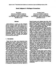
Proebsting 2009; Chen and Pennock 2007] 1 . Trading agents inform the quantity of a security they wish to buy or sell to the market maker. If a trading agent purchases δ units of a security, the market maker determines the payment the agent has to make as C(q + δ) − C(q). Correspondingly, if the agent sells δ quantity of the security, it receives a payoff of C(q) − C(q − δ) from the market maker. Figure 1 shows the main entities of a prediction market along with the operations performed by a trader (trading agent) in a prediction market and the portions of the prediction market that are affected by the partially observable stochastic game (POSG) representation described in the next section.

Fig. 1. The diagram showing the main entities of a prediction market where the partially observable stochastic game (POSG) representation is applied and the essential operations performed by a trading agent in a prediction market.

4. PARTIALLY OBSERVABLE STOCHASTIC GAMES FOR TRADING AGENT INTERACTION

We now describe our multi-agent prediction market model based on partially observable stochastic games. For simplicity of explanation, we consider a prediction market where a single security is being traded over a certain duration. This duration is divided into trading periods, with each trading period corresponding to a certain time period in a real prediction market. The ‘state’ of the market is expressed as the quantity of the purchased units of the security in the market. At the end of each trading period, each trading agent receives information about the state of the market from the market maker. With this prior information, the task of a trading agent is to determine a suitable quantity to trade for the next trading period, so that its utility is maximized. In this scenario, the environment of the agent is partially observable because other agents’ actions and payoffs are not known directly, but available through their aggregated beliefs. Agents interact with each other in trading periods (stages), and in each trading period the state of the market is determined stochastically based on the actions 1 Parameter b (determined by the market maker) controls the monetary risk of the market maker as well as the quantity of shares that trading agents can trade at or near the current price without causing massive price swings. Larger values for b allows trading agents to trade more frequently but also increases the market maker’s chances to lose money.


1:7

of all agents and the previous state of the prediction market. This scenario directly corresponds to the setting of a partially observable stochastic game (POSG) [Fudenberg and Tirole 1991; Hansen et al. 2004]. A partially observable stochastic game model offers several attractive features such as structured behavior by the agents by using best response strategies, stability of the outcome based on equilibrium concepts, lookahead capability of the agent to plan their actions based on future expected outcomes, ability to represent the temporal characteristics of the interactions between the agents, and, enabling all computations locally on the agents so that the system is robust and scalable. Previous research [Jumadinova and Dasgupta 2011b] has shown that information related parameters in a prediction market such as information availability, information reliability, information penetration, etc., have a considerable effect on the belief (price) estimation by trading agents and on the accuracy of the prediction market. Based on these findings, we posit that a component to model the impact of information related to an event should be added to the partially observable stochastic game framework in order to represent a prediction market accurately. With this feature in mind, we propose an interaction model called a partially observable stochastic game with information (POSGI) for capturing the strategic decision making by trading agents. A partially observable stochastic game with information (POSGI) is defined as: Γ = (N, S, (Ai )i∈N , (Ri )i∈N , T, (Oi )i∈N , Ω, (Ii )i∈N ), where N is a finite set of agents, S is a finite, non-empty set of states - each state corresponding to certain quantity of the security being held (purchased) by the trading agents. Ai is a finite non-empty action space of agent i s.t. ak = (a1,k , ..., a|N |,k ) is the joint action of the agents and ai,k is the action that agent i takes in state k, where agents take actions sequentially. In terms of the prediction market, a trading agent’s action corresponds to certain quantity of security it buys or sells, while the joint action corresponds to changing the purchased quantity for a security and taking the market to a new state. Ri,k is the reward or payoff for agent i in state k which is calculated using the logarithmic market scoring rule market maker. T : T (s, a, s′ ) = P (s′ |s, a) is the transition probability of moving from state s to state s′ after joint action a has been performed by the agents. Oi is a finite non-empty set of observations for agent i that consists of the market price and the information signal, and oi,k ∈ Oi is the observation agent i receives in state k. Ω : Ω(sk , Ii,k , oi,k ) = P (oi,k |sk , Ii,k ) is the observation probability for agent i of receiving observation oi,k in state sk when the information S signal is Ii,k . Finally, Ii is the information set received by agent i for an event Ii = k Ii,k where Ii,k ∈ {−1, 0, +1} is the information received by agent i in state k. The complete information arriving S to the market I = i∈N Ii is temporally distributed over the duration of the event. Information that improves the probability of the positive outcome of the event is considered positive (Ii,k = +1) and vice-versa, while information that does not affect the probability is considered to have no effect (Ii,k = 0). For example, for a security related to the event “Obama to be re-elected as US president in 2012”, information about Governor Chris Christie giving high praise to Obama following New Jersey’s storm in 2012 would be considered high impact positive information and information about high unemployment numbers would be considered negative information.

4.1. Overview of POSGI framework and its components

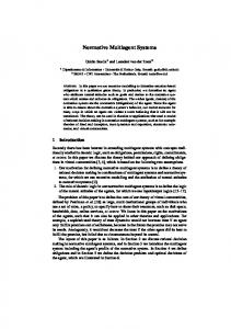
Our proposed partially observable stochastic game with information framework consists of the prediction market, the trading agents and the external information. Figure 2 shows the transition diagram based on the partially observable stochastic game with information formulation of the prediction market representing the interaction of the ACM Transactions on Embedded Computing Systems, Vol. 1, No. 1, Article 1, Publication date: August 2014.

1:8

Fig. 2. A diagram showing the interactions of the trading agent with the prediction market and the external information sources. The diagram shows representation for one agent i.

trading agent with the prediction market and information sources 2 . The prediction market (environment) goes through a set of states S˜ = {s1 , ..., sH } : S˜ ∈ S, where H is the duration of the event in the prediction market and sh represents the state of the market during trading period h. This state of the market is not visible to any agent, agents can only observe past states. However, each agent i has its own internal belief state Bi,h corresponding to its belief about the actual state sh . Bi,h gives a probability distribution over the set of states S, where Bi,h = (b1,h , ..., b|S|,h). At each trading period h, trading agent i takes an action ai,h , which could be either to buy, sell or hold a certain quantity of a security corresponding to a particular event in the prediction market; the corresponding joint action of the agents is denoted by ah = (a1,h , a2,h ...). Depending on the overall quantities of a security that have been bought or sold at trading period h, or, in other words, depending on this joint action of the agents, the state of the prediction market changes from sh to sh+1 , defined by the state transition function T (sh , ah , sh+1 ), and, the market price is updated. The agent i, however, doesn’t directly see the new state, but instead receives an observation oi,Sh+1 = (πsh+1 , Ii,sh+1 ), that includes the market price πsh+1 corresponding to the state sh+1 as informed by the market maker, and the information signal Ii,sh+1 . In order to make a decision to buy, sell or hold a certain quantity of the security, the trading agent i updates its beliefs using our proposed belief update function by accounting for the observation it received, its past belief, and its past action, as discussed in Section 4.2. Finally, agent i selects an action using an action selection strategy and receives a reward Ri,sh . The action selection strategy that we propose is based on a correlated equilibrium, where a trusted third party calculates the correlated equilibrium and recommends an action to each agent following this equilibrium. The details of the correlated equilibrium algorithm and some theoretical results are described in Section 4.4. 2 We only show one agent i to keep the diagram legible, but the same representation is valid for every agent in the prediction market.


1:9 4.2. Trading agent belief update and utility functions

A belief state of a trading agent is a probability vector that gives a distribution over the set of states S in the prediction market, i.e. Bi,h = (b1,h , ..., b|S|,h ), as previously discussed in Section 4. A trading agent uses its belief update function b : ℜ|S| × Ai × Oi → ℜ|S| to update its belief state based on its past action ai,h−1 , past belief state Bi,h−1 and the observation oi,Sh . The calculation of the belief update function for each element of the belief state, bs′ ,h , s′ ∈ S, is described below: P (s′ , ai,h−1 , oi , ) P (ai,h−1 , oi ) P (oi |s′ , ai,h−1 ) · P (s′ , ai,h−1 ) = P (oi |ai,h−1 )P (ai,h−1 )

bs′ ,h = P (s′ |ai,h−1 , oi ) =

(1)

Because ai,h−1 is conditionally independent given s′ and oi is conditionally independent given ai,h−1 , we can rewrite Equation 1 as: P (oi |s′ ) · P (s′ , ai,h−1 ) bs′ ,h = = P (oi )P (ai,h−1 ) P P ′ ′ s∈S P (s)P (s |s, ai,h−1 )P (ai,h−1 ) ι∈I P (ι)P (oi |s , ι) P (oi )P (ai,h−1 ) P P ′ ′ s∈S P (s)P (s |s, ai,h−1 ) ι∈I P (ι)P (oi |s , ι) = P (oi ) P P ′ ′ ι∈I P (ι)Ω(s , ι, oi ) s∈S T (s, ai,h−1 , s )bs,h−1 = P (oi )

(2)

All the terms in the r.h.s. of the Equation 2 can be calculated by an agent: P (ι) is the probability of receiving information signal ι, Ω(s′ , ι, oi ) is the probability of receiving observation oi in state s′ when the information signal is ι, T (s, ai,h−1 , s′ ) is the probability that the state s transitions to state s′ after agent i takes action ai,h−1 that agent can calculate using its knowledge of the current state and its past action, bs,h−1 is the past belief of agent i about state s, P (oi ) is the probability of receiving observation oi , which is a normalizing constant. Incorporating the risk preferences of the trading agents is an important factor in prediction markets. For example, the erroneous result related to the non-correlation between the trader beliefs and market prices in a prediction market in [Manski 2006] was because the risk preferences of the traders were not accounted for, as noted in [Gjerstad 2005]. This problem is particularly relevant for risk averse traders because the beliefs(prices) and risk preferences of traders have been reported to be directly correlated [Dimitrov and Sami 2010; Kadane and Winkler 1988]. Therefore, in our model we assume that the trading agents are risk-averse. The risk preference of an agent i is modeled through a utility function called the constant relative risk aversion. We use the constant relative risk aversion utility function to model risk averse agents because it allows to model the effect of different levels of risk aversion and it has been shown to be a better model than alternative families of risk modeling utilities [Wakker 2008]. It has been widely used for modeling risk aversion in various domains including economic domain [Holt and Laury 2002], psychology [Luce and Krumhansi 1988] and in the health domain [Bleichrodt et al. 1999]. The constant relative risk aversion utility function, ui (φ, Ri ), for agent i (for legibility we have dropped state k, ACM Transactions on Embedded Computing Systems, Vol. 1, No. 1, Article 1, Publication date: August 2014.

1:10

but the same calculation applies at every state) is given below: Ri1−θi , if θi = 6 1 1 − θi = ln(Ri ), if θi = 1

(3)

ui (φ, Ri ) =

Here, −1 < θi < 1 is called the risk preference factor of agent i with θi > 0 for riskaverse agents and Ri is the payoff or reward to agent i calculated using the logarithmic market scoring rule as was discussed in Section 3. The reward Ri is calculated after agent i’s trade is executed. When Ri < 0, we may get a utility in the form of a complex number. In that case, we convert the complex number to a real number by calling an existing function that uses magnitude and the angle of the complex number for conversion. 4.3. Trading agent action selection strategy

0, 0

...

q+4

+1,-1 -1,+1 +1,+1

0, 0 +1,-1 -1,+1

q+2

q-2

+1,-1 +1,+1

-1,-1 +1,0 0,+1

-1,0 0,-1

0,+1 +1,0

q +1,0

0,+1

...

-1,0 0,-1

q+3

0,+1 +1,0

-1,0 0,-1

-1,0 0,-1

q+1

+1,+1 0,0

+1,-1

-1,+1

q-3

...

-1,-1

-1,-1

+1,+1

...

0,0 -1,+1

-1,-1

+1,+1 +1,0 0,+1

q-4

-1,-1

q-1 0,0 -1,+1 +1,-1

Fig. 3. Finite state automata of the environment with two agents represented by the number of outstanding units of the security, q, in the prediction market. Based on the set of actions available to each agent, the state can transition to one of the following states: q + 2 (both agents buy), q + 1 (only one agent buys), q (both agents hold, or, one agent buys while the other agent sells, resulting in no transition), q −1 (only agent sells), and q − 2 (both agents sell).

The objective of a trading agent in a prediction market is to select an action at each trading period so that the expected utility that it receives is maximized. To understand this action selection process, we consider the decision problem facing each trading agent. As an example consider two agents whose available actions during each time step are to buy (=+1) or sell(=-1) only one unit of the security or not do anything (=0) by holding the security. Let the market state be denoted by q, the number of purchased units of the security. Based on the set of actions available to each agent, the state can transition to one of the following states q + 2 (both agents buy), q + 1 (only one agent buys), q (both agents hold, or, one agent buys while the other agent sells, resulting in no transition), q − 1 (only agent sells), and q − 2 (both agents sell), as shown in Figure 3. We can expand this state space further by adding more states and transitions, but the number of states remains finite because the set of states S of the partially observable stochastic game with information is finite. Also, since the number of units of a security ACM Transactions on Embedded Computing Systems, Vol. 1, No. 1, Article 1, Publication date: August 2014.

1:11

is finite, the number of securities the trading agent is allowed to buy or sell is bounded and the number of transitions from a state is guaranteed to be bounded. We also do not consider budget restrictions for the trading agents in this work. 4.4. Correlated Equilibrium (CE) calculation

In the partially observable stochastic game with information, the aggregated price information received by a trading agent from the market maker can be treated as a recommendation signal for selecting the agent’s strategy. This situation lends itself to a correlated equilibrium (CE) [Aumann 1974; Papadimitriou and Roughgarden 2008], where a trusted external agent privately recommends a strategy to play to each player. A correlated equilibrium is more preferred to the Nash or Bayesian Nash equilibrium because it can lead to improved payoffs, and it can be calculated using a linear program in time polynomial in the number of agents and number of strategies. Each agent i has a finite set of strategy profiles, Φi defined over its action space Ai . Q|N | Q The joint strategy space is given by Φ = i=1 Φi and let Φ−i = j6=i Φj . Let φ ∈ Φ denote a strategy profile and φi denote player i’s component in φ. A correlated equilibrium is a distribution p on Φ such that for all agents i and all strategies φi , φ′i if all agents follow a strategy profile φ that recommends player i to choose strategy φi , agent i has no incentiveP to play another strategy φ′i instead. This implies that the following expression holds: φ−i ∈Φ−i p(φ)(ui (φ) − ui (φ′i , φ−i )) ≥ 0, ∀i ∈ N , ∀φi , φ′i ∈ Φi and where ui (φ′i , φ−i ) is the utility that agent i gets when it changes its strategy to φ′i while all the other agents keep their strategies fixed at φ−i and p(φ) is the probability of realizing a given strategy profile φ. We now prove the existence of a correlated equilibrium in our prediction market based on a partially observable stochastic game with information. T HEOREM 4.1. A correlated equilibrium (CE) exists in our prediction market based on the partially observable stochastic game with information representation at each stage (trading period). P ROOF. At each stage in our prediction market, we can specify the correlated equilibrium by means of linear constraints as given below: X

p(φ)(ui (φ) − ui (φ′i , φ−i )) ≥ 0, ∀i ∈ N, ∀φi , φ′i ∈ Φi

(4)

φ−i ∈Φ−i

X

(5)

p(φ) = 1,

φ∈Φ

(6)

p(φ) ≥ 0

Equation 4 states that when agent i is recommended to select strategy φi , it must get no less utility from selecting strategy φi as it would from selecting any other strategy φ′i . Constraints given in Equations 5 and 6 guarantee that p is a valid probability distribution. We can rewrite the linear program specification of the correlated equilibrium above by adding an objective function to it. X X max p(φ), or min − p(φ) s.t. (7) φ∈Φ

X

φ∈Φ

p(φ)(ui (φ) − ui (φ′i , φ−i )) ≥ 0,

φ∈Φ,φ−i ∈Φ−i


(8)

1:12

(9)

p(φ) ≥ 0

Equation 8 is either trivial with a maximum of 0 or unbounded. Next, we show the relationship between Equation 5, which defines correlated equilibrium in the form of a constraint program, and the alternate formulation of this problem given in Equation 8. L EMMA 4.2. Problem given in Equation 5 has a solution iff problem in Equation 8 is unbounded. P ROOF. If problem in Equation 5 has a solution p(φ), then p(φ) is also feasible in the problem given in Equation 8. However, since for any a > 1 ap(φ) is also feasible in EquationP8, but it has a larger value, p(φ) is not optimal solution in Equation 8. Thus, lima→∞ φ∈Φ (ap(φ)) = ∞ and therefore problem in Equation 8 is unbounded. If the problem in Equation 8 is unbounded, its set of solutions is non-empty (by definition). We can transform an arbitrary solution p′ (φ) 6= 0 into a solution p(φ) for problem in Equation 5 by normalizing to guarantee that p(φ) is a valid distribution. QED. Lemma 4.2 shows that there is a correlated equilibrium if and only if problem in Equation 8 is unbounded. To prove the unboundedness we consider the dual problem of Equation 8 given in Equation 11. max 0, s.t. X

(10)

p(φ)[(ui (φ) − ui (φ′i , φ−i )]T ≤ −1

(11)

φ∈Φ,φ−i ∈Φ−i

(12)

p(φ) ≥ 0 ui (φ′i , φ−i )]p(φ)

= 0. where for every p(φ) there is p(φ) such that p(φ)[(ui (φ) − In [Papadimitriou and Roughgarden 2008], the authors showed that the problem given in Equation 11 is infeasible. From operations research we know that when the dual problem is infeasible the primal problem is feasible and unbounded. This means that the primal problem from Equation 8 is unbounded. We can then conclude that there is at least one correlated equilibrium in every trading period of the prediction market. We note that although the constant relative risk aversion utility function is concave, the concave structure does not affect the existence of at least one correlated equilibrium because the unboundedness of Equation 8 is not affected by the concave structure of ui . QED. To calculate correlated equilibrium(CE) we first characterize the set of all Pareto optimal strategy profiles. A strategy profile φP is Pareto optimal if there does not exist another strategy profile φ′ such that ui (φ′ ) ≥ ui (φP ) ∀i ∈ N with at least one inequality strict. In other words, a Pareto optimal strategy profile is one such that no trader could be made better off without making someone else worse off. A Pareto optimal strategy profile can be found by maximizing weighted utilities maxφ

|N | X

λi ui (φ) for some λi

(13)

i=1

Setting λi = 1 for all i ∈ N gives a utilitarian social welfare function. The maximization problem in Equation 13 can be solved using the Lagrangian method. We get the ACM Transactions on Embedded Computing Systems, Vol. 1, No. 1, Article 1, Publication date: August 2014.

1:13

following system of |N | equations: |N | X i=1

λi

ui (φ) = 0 , ∀j = 1, ..., |N | φi

(14)

that must hold at φP . Each of these equations is obtained by taking a partial derivative of the respective agent’s weighted utility with respect to respective agent’s strategy profile, thus solving the maximization problem given in Equation 13. By solving the system of equations 14 we get the set of Pareto optimal strategy profiles, ΦP . We then apply the correlated equilibrium calculation algorithm shown in Algorithm 1 on ΦP . Algorithm 1 is based on the Ellipsoid Against Hope algorithm proposed by [Papadimitriou and Roughgarden 2008]. We have used the correction proposed by Stein et al. [Papadimitriou and Roughgarden 2012] to solve the numerical precision problems that might arise in the Ellipsoid Against Hope algorithm. The calculation of the matrix values of the U matrix must be done once for each of the N agents. The computation 2 of the utility difference ui (φ) − ui (φi , φ−i ) for each agent i can be done in |ΦP i | time. Therefore, the time complexity of the CECalc algorithm during each trading period 2 comes to N × |ΦP i | . Since we consider securities that are independent (not correlated), the correlated equilbrium algorithm itself will not be affected as the number of securities increase. However, the computation time required by an agent, handling computation related to multiple securities will increase linearly as the number of securities increase. algorithm 1: Correlated Equilibrium Algorithm CECalc(D, ΦP ) Input: D, ΦP //D is the duration of the market, ΦP is the set of Pareto optimal strategies Output: p //correlated equilibrium foreach t ← 0 to D do //do this in each trading period Let U be the matrix consisting of the values of (ui (φ) − ui (φi , φ−i )), ∀i ∈ N, φ ∈ ΦP , φ−i ∈ ΦP i p′t ← getDualDistribution(ΦP , U ); pt ← solve for pt s.t. pt U T p′t = 0; return pt ; end GetDualDistribution(ΦP , U ) Input: ΦP , U Output: ∆ l = 0; p′l ∈ [0, 1]; ∆ = {}; while U T · p′l ≤ −1 is feasible do ∆ = ∆ + p′l ; p′l+1 = pl + ǫN ; //increase all elements of p′ by some small amounts from vector ǫN l + +; end return ∆;

P ROPOSITION 4.3. If p is a correlated equilibrium and φ is a Pareto optimal strategy profile calculated by p in a prediction market with risk averse agents, then the strategy profile φP is incentive compatible, that is each agent is best off reporting truthfully. ACM Transactions on Embedded Computing Systems, Vol. 1, No. 1, Article 1, Publication date: August 2014.

1:14

P ROOF. We prove by contradiction. Suppose that φP is not an incentive compatible strategy, that is, there is some other φ′ for which ui (φ′ ) ≥ ui (φP )

(15)

Equation 15 violates two properties of φP . First of all, since φP is Pareto optimal, we know that Equation 15 is not true, since ui (φP ) ≥ ui (φ′ ) by the definition of Pareto optimal strategy profile. Secondly, if we rewrite Equation 15 as ui (φP ) − ui (φ′ ) ≤ 0 and multiply both sides by p(φP ), we get p(φP )[ui (φP ) − ui (φ′ )] ≤ 0. Since p is a correlated equilibrium this inequality can not hold, otherwise it would violate the definition of the correlated equilibrium. QED. 5. EXPERIMENTAL RESULTS

We have conducted several simulations using our partially observable stochastic game with information prediction market. The main objective of our simulations is to test whether there is a benefit to the agents to follow the correlated equilibrium strategy. We do this by analyzing the utilities of the agents and the market price. We consider events that are disjoint (non-combinatorial). This allows us to compare our proposed strategy empirically with other existing strategies while using real data collected from the Intrade prediction market, which also considers non-combinatorial events. We report the market price for the security corresponding to the outcome of the event occurring. We assume that risk aversion coefficient of our trading agents, θ = 0.6, unless specified otherwise, since experimental evidence suggests that this value captures humans’ risk attitude without being too extreme in either direction [Goeree et al. 2003]. Since currently there is no real data relating to the risk averseness of the human traders and our main goal is to demonstrate the performance of our algorithm, we assume that the trading agents all have the same level of risk aversion. 5.1. Intrade Data Table I. Intrade markets used for our experiments. Name

Description

Presidential Election Recession

“Barack Obama to be elected President in 2008” “The US economy to go into recession in 2008” “The Social Network to win Best Picture 2011” “Lee DeWyze to win American Idol (Season 9)”

Best Picture American Idol

Total number of traders 3252

Total number of securities traded 1, 244, 892

Duration (Trading period) 744 days

728

75, 187

600 days

242

18,767

142 days

105

17,292

93 days

For all of our experimental results we have used commercially available data from four diverse prediction markets obtained from Intrade [Intrade 2012] company. The details of the Intrade markets that were used for our experiments are given in Table I and the market prices of these markets in Intrade are shown in Figure 4.We note that the date format that is used in Intrade’s data and shown in our graphs is day/month/year. We have obtained the general market data comprising of the market price data for each day and also the trade data consisting of the number of shares bought and sold by individual traders and the changes in price after each trade. Intrade prediction market allows for two possible outcomes to each event - yes, the event will happen as described, or no, it will not happen. Intrade is an exchange, so each ACM Transactions on Embedded Computing Systems, Vol. 1, No. 1, Article 1, Publication date: August 2014.

1:15 100

100

2010 American Idol

2010 Best Picture

90

80

80

70

70

Market Price

Market Price

90

60 50 40 30 20

60 50 40 30 20

10

10

0 0 (23/02/2010)

93 (27/05/2010)

0 (09/10/2010)

Number of days (since the start)

a

b

100

100

2008 Recession

90

2008 Presidential Elections

90

80

80

70

70

Market Price

Market Price

142 (28/02/2011)


60 50 40 30 20

60 50 40 30 20

10

10

0 (02/08/2007)

600 (24/03/2009)


c

0 (23/10/2006)

744 (05/11/2008)


d

Fig. 4. Actual market prices of the American Idol(a), Best Picture(b), Recession(c), and Presidential Elections(d) Intrade markets.

Fig. 5. The modified diagram showing the main entities of a prediction market and the essential operations performed by a trading agent in a prediction market with the Intrade market prices, Google news information signals, and the logarithmic market scoring rule (LMSR) market maker used in our experiments labeled appropriately.

trader buys or sells securities from another member of Intrade. Therefore, for our experiments we assume that the market maker in our model only calculates the market price and the trading agents’ rewards, but does not sell or buy securities itself. In Intrade when the market’s outcome becomes known, the market settles at either $0 or $10. If the market’s event happens, the traders holding securities corresponding to the market get paid $10 for every security that they hold. If the market’s event does not happen, the traders with the securities of that market do not get anything. Also, since Intrade allows short selling, i.e. selling securities that you don’t yet own, we also allow ACM Transactions on Embedded Computing Systems, Vol. 1, No. 1, Article 1, Publication date: August 2014.

1:16

short selling in our simulated partially observable stochastic game with information market. In all of our simulations we have used the same number of trading agents as the number of traders in Intrade markets, and we have also synced the start, trade and end times of our trading agents in each simulated market with the start, trade and end times of the real traders from Intrade markets. Figure 5 is a modified Figure 1 indicating the inputs to and outputs of our partially observable stochastic game with information prediction market model used for our simulations. Trading agents receive Intrade’s market price according to time steps indicated in the Intrade’s data. The market price in Intrade is updated after each trade. We have conducted two types of experiments, in the first type of experiments we compare the utility from correlated equilibrium strategy with the utility from the Intrade market, and in the second type of experiments we compare the correlated equilibrium strategy to other well-known strategies. For the first type of experiments, in order to be able to compare with the Intrade’s data we assume that the trading agents receive Intrade’s market price instead of the logarithmic market scoring rule market price, but they use the correlated equilibrium strategy to determine their action and receive utility based on it. For the second type of experiments, we assume that the market maker uses the logarithmic market scoring rule to calculate the market price as specified in the partially observable stochastic game with information model. We have used Google News [News 2012] to obtain information signals that the trading agents receive. We have used each market’s description as specified by Intrade, to obtain results in Google News, which were narrowed down by the time period during which each market was active. The results were then ran through SentiStrength [Thelwall et al. 2010], which is a tool that estimates the strength of positive and negative sentiment in short texts. We have specified positive strength sentiment to be 1, negative strength sentiment to be −1, and neutral strength sentiment to be 0. SentiStrength basically gives a score (1, −1 or 0) to each result obtained from Google News, which is then used as an information signal sent to a number of the trading agents selected randomly from the total agent population at the same time step (date and time) as the date and time it was published on Google News. Finally, the trading agents in our model update their beliefs either when they receive a new information signal or at the belief update time step interval, which is determined as an average trading time of all traders in the market. We noticed that there were different kind of traders in the Intrade markets, for example some traders were very active and some were not very active, some traders only joined the market for 1 day and some traded in the market throughout its duration. Therefore in order to analyze the performance of different types of trading agents, we have clustered the traders in each of four Intrade markets that we have used according to the duration of their participation in the market and the number of their trades. We used EM(expectation maximization) clustering technique [Dempster et al. 1977] within a popular clustering tool, called Weka 3.6 [Hall et al. 2009]. We didn’t specify the number of clusters, instead EM used cross validation to select the number of clusters automatically. We obtained 3 clusters for the American Idol and 3 clusters Best Picture markets, 4 clusters for the Recession market, and 4 clusters for the Presidential Election market. For our first set of experiments, we want to compare the performance of the trading agents using the correlated equilibrium strategy within partially observable stochastic game with information model with the performance of the traders in the real Intrade market. We ran simulations of our partially observable stochastic game with information model where all trading agents use the correlated equilibrium strategy and we compare their utility to the utility of the actual traders in the Intrade markets using ACM Transactions on Embedded Computing Systems, Vol. 1, No. 1, Article 1, Publication date: August 2014.

1:17 60

2000

1500

1000

40

CE

Intrade

1000

0 20

-20

CE

500

Utility

Intrade

0

Utility

Utility

-1000 -2000 -3000

CE 0

-4000 -40

Intrade -5000

-60

-500

-6000

36 (31/03/2010)

71 (05/05/2010)

8 (03/03/2010)


85 (27/05/2010)

0 (23/02/2010)


a

93 (27/05/2010)


b

c

Fig. 6. Average cumulative utilities of the traders in Intrade markets and the trading agents in the partially observable stochastic game with information (POSGI) prediction market for clusters 1 (a), 2 (b), and 3 (c) in the American Idol market. We observe that the trading agents using the correlated equilbrium (CE) strategy are able to get more utility than the human traders in the American Idol Intrade market. 300 200

600

CE

1000

CE Intrade

500

100

400 0

Utility

Utility

Utility

0 200

-100

-500

-200

0

Intrade CE

-300

Intrade

-1000

-200 -400

108 (25/01/2011)

129 (15/02/2011)

-1500

14 (23/10/2010)

139 (25/02/2011)

0 (09/10/2010)

142 (28/02/2011)




a

b

c

Fig. 7. Average cumulative utilities of the traders in Intrade markets and the trading agents in partially observable stochastic game with information prediction market for clusters 1 (a), 2 (b), and 3 (c) in the Best Picture market. We observe that the trading agents using the correlated equilbrium (CE) strategy are able to get more utility than the human traders in the Best Picture market.

Equation 4. We show the results for the average cumulative utility of the traders in Intrade market and the average cumulative utility of the trading agents in the partially observable stochastic game with information market for each cluster in each market. The last point in the utility graphs corresponds to the final utility that the trading agents receive after the market clears, i.e. trading agents get paid $10 for each security they possess at the end of the market. Figures 6 and 7 (a-c) show the average cumulative utility of the trading agents for cluster 1, 2, and 3 correspondingly in the American Idol and the Best Picture markets. While Figures 8 and 9 (a-d) show the average cumulative utility of the trading agents for cluster 1, 2, 3, and 4 correspondingly in the Recession and the Presidential Election markets. We note that different clusters have different durations, for example in the Best Picture market, cluster 1 shown in Figure 7(a) lasts for only 21 days, whereas cluster 3 shown in Figure 7(c) lasts for the entire duration of the market. From this set of experiments we observe that due to the look-ahead capability of the correlated equilibrium strategy the trading agents are able to get more utility than the human traders in the Intrade markets. One of the reasons for a negative trading agents’ utility throughout most of the duration in some markets is because the agents buy securities at the beginning of the market’s duration and in the markets(or clusters) with a shorter duration, such as the American Idol market, they do not have enough time to play the market to increase their utility until almost the end of the market. However, in the markets with longer duration the trading agents are able to increase their ACM Transactions on Embedded Computing Systems, Vol. 1, No. 1, Article 1, Publication date: August 2014.

1:18

200

700 600

150

500 400

100

Utility

Utility

300 50

CE

0

200 100

Intrade

0 -50

-100

Intrade

-200

-100

CE

-300 229 (18/03/2008)

242 (31/03/2008)

298 (26/05/2008)


519 (02/01/2009)


a

b

1500 1500 1000

Utility

Utility

Intrade

0

CE

1000

CE 500

500

Intrade

0 -500 -500 65 (06/05/2008)

600 (24/03/2009)


c

0 (02/08/2007)

383 (23/10/2008)


d

Fig. 8. Average cumulative utilities of the traders in Intrade markets and the trading agents in partially observable stochastic game with information (POSGI) prediction market for clusters 1 (a), 2 (b), and 3 (c) in the Recession market. We observe that the trading agents using the correlated equilbrium (CE) strategy are able to get more utility than the human traders in the the Recession market.

utility throughout the market’s duration. Another reason for the difference in the dynamics of the utility between various clusters is because traders’ trading behavior may also be different in different clusters. For example, in one cluster traders maybe more active and trade more often than in other clusters, leading cluster trader population to different utilities. From our experiments we observe that the duration of the prediction market, as well as trading volume and the trader population are important factors that determine the level of success of the correlated equilibrium strategy. The correlated equilibrium strategy seems to perform better in most cases when the duration of the prediction is longer since it allows the traders to use the strategy’s lookahead capability better. In summary of this set of experiments, we observe that using trading agents with the correlated equilibrium strategy to trade on behalf of humans may be beneficial since it leads to higher utility and it can avoid inefficient human trading decisions that might result in a very large loss, such as the one observed in the Presidential Election market for cluster 3 shown in Figure 9 (c). 5.2. Risk behavior of the trading agents

Next, we conduct experiments to compare trading agents’ behavior with different risk attitudes. To model the effect that different risk behaviors have on the prediction market, we vary the risk-aversive level (coefficient) of the trading agents from θ = 0.3 to ACM Transactions on Embedded Computing Systems, Vol. 1, No. 1, Article 1, Publication date: August 2014.

1:19

150

500

CE

100 0

Intrade

Utility

Utility

50 0 -50

-500

-1000

Intrade

CE

-100

-1500 -150

493 (28/02/2008)

590 (04/06/2008)

0 (22/11/2007)


744 (05/11/2008)


a

b

4

x 10 0

5000

CE

CE -0.5

Utility

Utility

0 -1

-1.5

Intrade

-5000

-10000

Intrade

-2 -15000 221 (01/06/2007)

743 (04/11/2008)

129 (01/03/2007)


744 (05/11/2008)


c

d

Fig. 9. Average cumulative utilities of the traders in Intrade markets and the trading agents in the partially observable stochastic game with information (POSGI) prediction market for clusters 1 (a), 2 (b), and 3 (c) in the Presidential Election market. We observe that the trading agents using the correlated equilbrium (CE) strategy are able to get more utility than the human traders in the in the Presidential Election market.

300

θ=0.3 θ=0.6

400

θ=0.6 θ=0.8

200

0

Utility

Utility

200

400

θ=0.3 θ=0.6 θ=0.8

-200 -400

200

Utility

400

100

0 -200

0

-400

-600 -100 -600 0 (02/08/2007) 600 (24/03/2009) 0 (02/08/2007) 600 (24/03/2009) 0 (02/08/2007) 600 (24/03/2009) Number of days (since the start) Number of days (since the start) Number of days (since the start)

a

b

c

Fig. 10. Average cumulative utilities of the agents with different risk factors in the Recession market. In Figure 10(a) the agent population is divided equally into three clusters with each cluster having a different risk aversive level. In Figures 10(b) and (c) the agent population is equally divided into agents with different risk aversion coefficients. We observe that the agents who are more risk averse (θ = 0.8) receive less utility than the agents who are less risk-averse (θ = 0.3 or θ = 0.6).

θ = 0.6 to θ = 0.8. In an experiment shown in Figure 10(a) we assume that the agent population is divided equally into three clusters with each cluster having a different risk aversive level. While in Figures 10(b) and (c) the agent population is equally diACM Transactions on Embedded Computing Systems, Vol. 1, No. 1, Article 1, Publication date: August 2014.

1:20

vided into agents with different risk aversion coefficients. We observe that the agents who are more risk averse (θ = 0.8) receive less utility than the agents who are less risk-averse (θ = 0.3 or θ = 0.6). This is because a more risk averse agents may hold back from making definite buying or selling decisions. This is also evidenced from Figure 10(b) where more risk averse agents with θ = 0.8 get 64% less utility than less risk averse agents with θ = 0.6. The concave nature of the constant relative risk aversion utility function with larger θ values lowers the utilities that these agents receive. The effect of the lowered utility due to the risk averse (concave) utility function is also seen in Figures 10(c). From here on we continue to use a risk aversion coefficient of θ = 0.6, as recommended by the literature [Goeree et al. 2003]. 5.3. Comparison with existing trading strategies

For our next set of experiments, we compare the trading agents’ and market’s behavior under various strategies employed by the trading agents in Intrade’s markets given in Table I. In this set of experiments in each run of each market all agents use the same trading strategy. We then compare separate runs with different strategies. We use the following five well-known published strategies for comparison with our proposed correlated equilibrium strategy. (1) ZI (Zero Intelligence) [Othman 2008] - each agent submits randomly calculated quantity to buy or sell. (2) ZIP (Zero Intelligence Plus) [Cliff 1997] - each agent selects a quantity to buy or sell that satisfies a particular level of profit by adopting its profit margin based on past prices. (3) CP (by Preist and Tol) [Ma and Leung 2008] - each agent adjusts its quantity to buy or sell based on past prices and tries to choose that quantity so that it is competitive among other agents. (4) GD (by Gjerstad and Dickhaut) [Ma and Leung 2008] - each agent maintains a history of past transactions and chooses the quantity to buy or sell that maximizes its expected utility. (5) DP (Dynamic Programming solution for the partially observable stochastic game) [Hansen et al. 2004] - each agent uses dynamic programming solution to find the best quantity to buy or sell that maximizes its expected utility given past prices, past utility, past belief and the information signal. In order to compare the effect of different trading strategies on the market prices, in the remaining set of experiments we have logarithmic market scoring rule market maker calculate the market price and send the logarithmic market scoring rule market price back to the trading agents instead of the Intrade’s market price. We first compare the market prices calculated by the logarithmic market scoring rule market maker and the real Intrade’s market prices. Table II shows the results of the t-test for hypothesis: Intrade and the logarithmic market scoring rule (LMSR)/partially observable stochastic game with information (POSGI) do not differ in terms of their mean market prices. Since the p values for all four markets are greater than 0.05, it means that there is no difference between the means of the Intrade and the logarithmic market scoring rule market prices. This indicates a strong correlation between the two market prices for all four prediction markets. Figures 11(a)-14(a) show the market prices calculated by the logarithmic market scoring rule market maker for four Intrade markets. In these graphs we want to see how the market prices set by an automated market maker using different strategies vary across various trading strategies. We observe that agents using the correlated equilibrium strategy are able to trade at prices that are closer to the final outcome of the event, indicating that agents using the correlated equilibrium strategy are able ACM Transactions on Embedded Computing Systems, Vol. 1, No. 1, Article 1, Publication date: August 2014.

1:21

100

1000 CE 500

GD

DP

DP

CE

0

60

Utility

Market price

80

GD 40

-500 -1000 -1500

CP

ZIP

20 -2000 ZIP 0 (23/02/2010)

ZI

CP 93 (27/05/2010)

0 (23/02/2010)


93 (27/05/2010)


a

b

Fig. 11. The market prices(a) and the average cumulative utilities(b) of the agents under different trading strategies for American Idol market. In each run all agents use the same trading strategy in this market. The comparison across separate runs with different strategies is presented in this Figure. We observe that agents using the correlated equilbrium (CE) strategy are able to trade at prices that are closer to the final outcome of the event and obtain more utility on average at the end of the Americal Idol market than the agents following other strategies.

100

500

80

0 CE

60

Utility

Market price

CE DP

DP

GD 40

-500

ZIP GD

CP

-1000

20 CP

ZI

ZIP 0 (09/10/2010)

142 (28/02/2011)


a

0 (09/10/2010)

142 (28/02/2011)


b

Fig. 12. The market prices(a) and the average cumulative utilities(b) of the agents under different trading strategies for Best Picture market. In each run all agents use the same trading strategy in this market. The comparison across separate runs with different strategies is presented in this Figure. We observe that agents using the correlated equilbrium (CE) strategy are able to trade at prices that are closer to the final outcome of the event and obtain more utility on average at the end of the Best Picture market than the agents following other strategies.

to respond to other agents’ strategies and predict the aggregated price of the security more efficiently. This efficiency is further supported by the graph in Figures 11(b)14(b) that show the average cumulative utilities of the agents while using different strategies. The agent population was uniformly divided for different strategies. We see that the agents using the correlated equilibrium strategy are able to obtain 39% more utility on average than the agents following the next best performing strategy (dynamic programming - DP) and 137% more utility on average than the agents following the worst performing strategy (ZI) in all markets. We also observe that the daily performance of the compared trading strategies differs slightly market to market. For example in Figure 12(b), Best Picture Market, the average cumulative utility for the correlated equilibrium strategy is less than that of other strategies during the beginACM Transactions on Embedded Computing Systems, Vol. 1, No. 1, Article 1, Publication date: August 2014.

1:22 Table II. Correlation test conducted using two tailed type 3 t-test showing the correlation of the market prices in the Intrade markets and the market prices produced by the logarithmic market scoring rule in partially observable stochastic game with information prediction markets. Market Presidential Election Recession Best Picture American Idol

100

p value of the t-test 0.07 0.11 0.08 0.12

1000

CE

CE GD

GD 500 CP

DP

60 ZIP 40

20

DP

Utility

Market Price

80

CP

0

-500

-1000 ZI

0 (02/08/2007)

600 (24/03/2009)


a

0 (02/08/2007)

ZIP 600 (24/03/2009)


b

Fig. 13. The market prices(a) and the average cumulative utilities(b) of the agents under different trading strategies for Recession market. In each run all agents use the same trading strategy in this market. The comparison across separate runs with different strategies is presented in this Figure. We observe that agents using the correlated equilbrium (CE) strategy are able to trade at prices that are closer to the final outcome of the event and obtain more utility on average at the end of the Recession market than the agents following other strategies.

ning of the market. Intuitively, this behavior may occur due to the market’s duration and the look-ahead behavior of this strategy - during shorter markets the correlated equilbrium strategy may not have enough time initially to suggest the best action as it may not have had enough history of past actions and past belief states to make the best decision. In addition, the best strategy toward the end maybe to hold the securities and sell them at the end, leading to a smaller intermediary utility but larger final utility. Overall, we can say that using the partially observable stochastic game with information model allows the agent to avoid myopically predicting prices and use the correlated equilibrium to calculate prices more accurately and obtain higher utilities. For our final set of experiments, we further compare the correlated equilibrium strategy with other strategies by equally dividing the agent population in each market into two groups in the same simulation run - one group of agents using the correlated equilibrium strategy and the other group of agents using the compared strategy. The results are obtained using the data from the Recession market and are reported in Figure 15 (a-d). We can see that in each scenario the correlated equilibrium strategy outperforms other strategies. We observe that the trading agent using the correlated equilibrium strategy gets 106% more utility than the trading agent using the zero intelligence plus strategy in the market with trading agents using only zero intelligence plus and the correlated equilibrium strategies and 48% more utility than the trading agent using the next best dynamic programming strategy in the market with trading agents using only dynamic programming and the correlated equilibrium strategies. In ACM Transactions on Embedded Computing Systems, Vol. 1, No. 1, Article 1, Publication date: August 2014.

1:23

100

100

DP GD

0

80 CE 60

40

CP

GD

-100

Utility

Market price

CE DP

-200 -300

20 CP 0 (23/10/2006)

ZIP

ZIP

-400

744 (05/11/2008)


a

ZI

0 (23/10/2006)

744 (05/11/2008)


b

Fig. 14. The market prices(a) and the average cumulative utilities(b) of the agents under different trading strategies for Presidential Election market. In each run all agents use the same trading strategy in this market. The comparison across separate runs with different strategies is presented in this Figure. We observe that agents using the correlated equilbrium (CE) strategy are able to trade at prices that are closer to the final outcome of the event and obtain more utility on average at the end of the Presidential Election market than the agents following other strategies.

summary, the partially observable stochastic game with information model and the correlated equilibrium strategy result in better price tracking and higher utilities because they provide each agent with a strategic behavior while taking into account the observations of the prediction market and the new information of the events. 6. CONCLUSIONS AND FUTURE WORK

In this paper, we presented a multi-agent prediction market based on the partially observable stochastic game with the logarithmic market scoring rule market maker. We proved the existence of a correlated equilibrium in our partially observable stochastic game with information prediction market and proposed an algorithm that can be used to obtain the correlated equilibrium in the prediction market with risk averse agents. We have also conducted simulation experiments using four real market data obtained from the Intrade prediction market company. We have compared the partially observable stochastic game and the correlated equilibrium based trading strategy with five different trading strategies used in similar markets. We have empirically verified that when the agents follow a correlated equilibrium strategy they obtain higher utilities and the market prices are more accurate than when they use other compared trading strategies. Our results also showed that trading agents using our proposed correlated equilibrium trading strategy gets higher utility than the human traders and can avoid inefficient human trading decisions that might result in a very large loss. There are several aspects of our work that are worth further investigation. First of all, our proposed Algorithm 1 outputs a correlated equilibrium that is found first, to reduce computational costs. But in some cases there may be multiple correlated equilibria and it is worth investigating what improvements, if any, can be made to the utilities of the agents and the market price by selecting the ‘best’ correlated equilibrium instead of just using the first correlated equilibrium. Secondly, we have assumed that the market maker uses the logarithmic market scoring rule to calculate the rewards of the agents and the market price. However, the logarithmic market scoring rule has been recently shown to have some drawbacks [Othman and Sandholm 2010b], for example, the market maker can run at a loss which can be large and a single parameter b controls the loss bound, the level of liquidity, and the rate of adaptability to market ACM Transactions on Embedded Computing Systems, Vol. 1, No. 1, Article 1, Publication date: August 2014.

1:24

600

600

400

400 CE

200

Utility

Utility

200 0 -200

CE

0 -200

ZIP

-400

0 (02/08/2007)

CP

-400

600 (24/03/2009) 0 (02/08/2007)


a

b

400

400 CE

200

CE

200 0

Utility

0

Utility

600 (24/03/2009)


-200 -400

-200 -400

-600

-600

GD

0 (02/08/2007)

DP

600 (24/03/2009) 0 (02/08/2007)


c

600 (24/03/2009)


d

Fig. 15. Comparisons of the average cumulative utilities of the agents using correlated equilbrium (CE) strategy versus zero intelligence plus (ZIP) (a), CP by Preist and Tol (b), GD by by Gjerstad and Dickhaut (c), and dynamic programming (DP) (d) strategies. The agent population in each market was divided into two groups in the same simulation run. We observe that in each case the correlated equilibrium strategy outperforms other strategies.

shocks. Since the market maker’s strategy was not the main point of this work, we did not explore different market making strategies. However, the effect of using different market maker strategies (i.e. Bayesian [Brahma et al. 2012]) could be further explored. Also, in the future we are interested in investigating the prediction market equilibrium behavior under different agent coalition formations. Finally, we are interested in investigating the dynamics evolving from multiple prediction markets that interact with each other. REFERENCES A UMANN, R. 1974. Subjectivity and correlation in randomized strategies. Journal of Mathematical Economics 1, 1, 67 – 96. B ERG, H. AND P ROEBSTING, T. 2009. Hanson’s automated market maker. In The Journal of Prediction Markets. 45–59. B ETFAIR. 2012. Betfair. http://www.betfair.com/. B LEICHRODT, H., VAN R IJN, J., AND J OHANNESSON, M. 1999. Probability weighting and utility curvature in qaly-based decision making. Journal of Mathematical Psychology 43, 238–260. B RAHMA , A., C HAKRABORTY, M., D AS, S., L AVOIE , A., AND M AGDON -I SMAIL , M. 2012. A bayesian market maker. In Proceedings of the 13th ACM Conference on Electronic Commerce. EC ’12. 215–232.


1:25 C HEN, Y., D IMITROV, S., S AMI , R., R EEVES, D., P ENNOCK , D., H ANSON, R., F ORTNOW, L., AND G ONEN, R. 2009. Gaming prediction markets: Equilibrium strategies with a market maker. Algorithmica 58, 4, 930–969. C HEN, Y., M ULLEN, T., AND C HU, C. 2006. An in-depth analysis of information markets with aggregate uncertainty. Electronic Commerce Research 6, 2, 201–222. C HEN, Y. AND P ENNOCK , D. 2007. Utility framework for bounded-loss market maker. In Proceedings of the 23rd Conference on Uncertainty in Articifial Intelligence (UAI ’07). 49–56. C LIFF , D. 1997. Minimal-intelligence agents for bargaining behaviours in market-based environments. HP Labs Technical report, HPL-97-91. C OWGILL , B., W OLFERS, J., AND Z ITZEWITZ , E. 2008. Using prediction markets to track information flows: Evidence from google. Tech. rep., Dartmouth College, bocowgill.com/GooglePredictionMarketPaper.pdf. January. D EMPSTER , A., L AIRD, N., AND R UBIN, D. 1977. Maximum likelihood from incomplete data via the em algorithm. Journal of Royal Statist. Soc. Ser. B 39, 1, 1–38. D IMITROV, S. AND S AMI , R. 2008. Nonmyopic strategies in prediction markets. In Proceedings of the 9th ACM Conference on Electronic Commerce (EC). 200–209. D IMITROV, S. AND S AMI , R. 2010. Composition of markets with conflicting incentives. In Proceedings of the 11th ACM conference on Electronic commerce. EC ’10. 53–62. D IMITROV, S., S AMI , R., AND E PELMAN, M. 2009. Subsidized prediction markets for risk averse traders. In Proceedings of the 5th International Workshop on Internet and Network Economics. WINE ’09. 491–497. F EIGENBAUM , J., F ORTNOW, L., P ENNOCK , D., AND S AMI , R. 2005. Computation in a distributed information market. Theoretical Computer Science 343, 1-2, 114–132. F UDENBERG, D. AND T IROLE , J. 1991. Game Theory. MIT Press. G JERSTAD, S. 2005. Risks, aversions and beliefs in predictions markets. mimeo, University of Arizona. G OEREE , J., H OLT, C., AND PALFREY, T. 2003. Risk averse behavior in generalized matching pennies games. Games and Economic Behavior 45, 1, 97–113. G RUCA , T., B ERG, J., AND C IPRIANO, M. 2008. Incentive and accuracy issues in movie prediction markets. The Journal of Prediction Markets 2, 1, 29–43. H ALL , M., F RANK , E., H. G., P FAHRINGER , B., R EUTEMANN, P., AND W ITTEN, I. 2009. The weka data mining software: An update. ACM SIGKDD Explorations Newsletter 11, 1, 10–18. H ANSEN, E., B ERNSTEIN, D., AND Z ILBERSTEIN, S. 2004. Dynamic programming for partially observable stochastic games. In Proceedings of the 19th National Conference on Artificial Intelligence. 709–715. H ANSON, R. 2003. Combinatorial information market design. Information Systems Frontiers 5, 1, 105–119. H ANSON, R. 2007. Logarithmic market scoring rules for modular combinatorial information aggregation. Journal of Prediction Markets 1, 1, 3–15. H OLT, C. AND L AURY, S. 2002. Risk aversion and incentive effects. American Economic Review 92, 1644– 1655. HSE. 2012. Hollywood stock exchange. http://www.hsx.com/. I NTRADE. 2012. Intrade. http://www.intrade.com/. I YER , K., J OHARI , R., AND M OALLEMI , C. 2010. Information aggregation in smooth markets. In Proceedings of the 11th ACM conference on Electronic commerce. EC ’10. 199–206. J UMADINOVA , J. AND D ASGUPTA , P. 2011a. A multi-agent prediction market based on partially observable stochastic game. In Proceedings of the 13th International Conference on Electronic Commerce. ICEC ’11. 21:1–21:10. J UMADINOVA , J. AND D ASGUPTA , P. 2011b. A multi-agent system for analyzing the effect of information on prediction markets. International Journal of Intelligent Systems 26, 1, 383–409. J UMADINOVA , J. AND D ASGUPTA , P. 2011c. Partially observable stochastic game-based multi-agent prediction markets. In Proceedings of the 10th International Conference on Autonomous Agents and Multiagent Systems (AAMAS ’11), (short paper). 1217–1218. K ADANE , J. AND W INKLER , R. 1988. Separating probability elicitation from utilities. Journal of the American Statistical Association 83, 402, 357–363. L ITTMAN, M. 1994. Markov games as a framework for multi-agent reinforcement learning. In ICML. Vol. 94. 157–163. L UCE , R. AND K RUMHANSI , C. 1988. Measurement, scaling, and psychophysics. In Stevens Handbook of Experimental Psychology, Wiley: New York 1, 3–74. M A , H. AND L EUNG, H. 2008. Bidding Strategies in Agent-Based Continuous Double Auctions. Whitestein Series In Software Agent Technologies And Autonomic Computing.


1:26 M ANSKI , C. 2006. Interpreting the predictions of prediction markets. Economic Letters 91, 3, 425–429. N EWS, G. 2012. Google news. http://news.google.com. O STROVSKY, M. 2009. Information aggregation in dynamic markets with strategic traders. In Proceedings of the 10th ACM conference on Electronic commerce (EC’09). 253–254. O THMAN, A. 2008. Zero intelligence agents in prediction markets. In Proceedings of the 7th International Conference on Autonomous Agents and Multiagent Systems. 879–886. O THMAN, A. AND S ANDHOLM , T. 2010a. Automated market-making in the large: the gates hillman prediction market. In Proceedings of the 11th ACM conference on Electronic commerce. EC ’10. 367–376. O THMAN, A. AND S ANDHOLM , T. 2010b. When do markets with simple agents fail? In Proceedings of the 9th International Conference on Autonomous Agents and Multiagent Systems: Volume 1. AAMAS ’10. 865–872. O THMAN, A., S ANDHOLM , T., P ENNOCK , D., AND R EEVES, D. 2010. A practical liquidity-sensitive automated market maker. In Proceedings of the 11th ACM conference on Electronic commerce. EC ’10. 377– 386. PAPADIMITRIOU, C. AND R OUGHGARDEN, T. 2008. Computing correlated equilibria in multi-player games. Journal of ACM 1, 29, 14:1–14:29. PAPADIMITRIOU, C. AND R OUGHGARDEN, T. 2012. Comments on “computing correlated equilibria in multiplayer games”. http://stanford.edu/~ tim/papers/comment.pdf. P ENNOCK , D. AND S AMI , R. 2007. Computational aspects of prediction markets, In Algorithmic Game Theory. Cambridge University Press. N. Nisan, T. Roughgarden, E. Tardos, V. Vazirani, editors. P LOTT, C. AND C HEN, K. 2002. Information aggregation mechanisms: Concept, design and implementation for a sales forecasting problem. Tech. rep., Social Science working paper no. 1131, California Institute of Technology. March. S UROWIECKI , J. 2005. The wisdom of crowds. New York: Anchor Books. ISBN: 0-385-72170-6. S ZOLNOKI , A., WANG, Z., AND P ERC, M. 2012. Wisdom of groups promotes cooperation in evolutionary social dilemmas. Scientific Reports 2, 576. T HELWALL , M., B UCKLEY, K., PALTOGLOU, G., C AI , D., AND K APPAS, A. 2010. Sentiment strength detection in short informal text. Journal of the American Society for Information Science and Technology 61, 12, 2544–2558. WAKKER , P. 2008. Explaining the characteristics of the power (crra) utility family. Health Economics 17, 1329–1344. WANG, X., P ERC, M., L IU, Y., C HEN, X., AND WANG, L. 2012. Beyond pairwise strategy updating in the prisoner’s dilemma game. Scientific Reports 2, 740. W OLFERS, J. AND Z ITZEWITZ , E. 2004. Prediction markets. Journal of Economic Perspectives 18, 2, 107– 126.


1 Automated Pricing in a Multi-agent Prediction ... - Semantic Scholar

1 Automated Pricing in a Multi-agent Prediction ... - Semantic Scholar

Suggest Documents

Multiagent realization of prediction-based ... - Semantic Scholar

Automated Product Pricing Using Argumentation - Semantic Scholar

Automated Prediction of Temporal Relations - Semantic Scholar

An Automated Maintainability Prediction Tool ... - Semantic Scholar

Developing a Multiagent Conference Management ... - Semantic Scholar

A Secure Multiagent Intelligent Conceptual ... - Semantic Scholar

Commercializing a Multiagent-Supported ... - Semantic Scholar

Social Judgment in Multiagent Interactions - Semantic Scholar

Coordination in Multiagent Reinforcement Learning - Semantic Scholar

MASSPEC - MULTIAGENT SYSTEM ... - Semantic Scholar

Learning Conventions in Multiagent Stochastic ... - Semantic Scholar

Quantifying Privacy in Multiagent Planning - Semantic Scholar

Issues in Multiagent System Development - Semantic Scholar

Normative Multiagent Systems - Semantic Scholar

Cooperative Multiagent Learning - Semantic Scholar

Fuzzy Reasoning in a MultiAgent System of ... - Semantic Scholar

Bottom-Up/Top-Down Coordination in a MultiAgent ... - Semantic Scholar

Congestion Pricing - Semantic Scholar

AMPA: an automated web server for prediction of ... - Semantic Scholar

Automated Prediction of the Apnea-Hypopnea ... - Semantic Scholar

PFP/ESG: automated protein function prediction ... - Semantic Scholar

Performance Prediction and Automated Tuning of ... - Semantic Scholar

ExPlanTech: Multiagent Support for Manufacturing ... - Semantic Scholar

Muon: Designing Multiagent Communication ... - Semantic Scholar