WP-2006-012
Through a Glass Darkly: Deciphering the Impact of Oil Price Shocks
Ashima Goyal and Arjun Singh
Indira Gandhi Institute of Development Research, Mumbai December 2006
Through a Glass Darkly: Deciphering the Impact of Oil Price Shocks1 Ashima Goyal and Arjun Singh Indira Gandhi Institute of Development Research (IGIDR) General Arun Kumar Vaidya Marg Goregaon (E), Mumbai- 400065, INDIA Email (corresponding author):
[email protected],
[email protected] Abstract In order to examine if the impact of oil price shocks depends on the structure of an economy, a vertical (VSC) and a horizontal (HSC) long-run supply curve identification are successively imposed on a three variable VAR with Indian time series data. While core inflation is measured with the VSC, the HSC requires a new concept of demand-driven inflation: Residual (demand) inflation, which gives the impact of short and medium run demand shocks on inflation. Core and residual inflation are both estimated. The data favors the HSC, but both identifications imply that policy demand squeeze aggravated international oil price shocks. Key words: Oil Shocks, VAR, Identification strategies, Developing economy, Residual Inflation JEL Code(s): E31, C32
1
This paper extends Arjun Singh’s dissertation originally written under the guidance of Ashima Goyal. Comments received from Kausik Chaudhuri, Veena Mishra, D.M. Nachane, R. Radhakrishna, Naveen Srinivasan and Rajendra Vaidya are gratefully acknowledged.
2
Through a Glass Darkly: Deciphering the Impact of Oil Price Shocks Ashima Goyal and Arjun Singh 1. Introduction In order to examine if the impact of oil price shocks, on inflation and output, depends on the structure of an economy, a vertical (VSC) and a horizontal (HSC) long-run supply curve identification are successively imposed on a three variable VAR with Indian time series data. While core inflation is measured with the VSC, the HSC requires a new concept of demand-driven inflation: Residual (demand) inflation, which gives the impact of short and medium run demand shocks on inflation. Simultaneity among macroeconomic variables implies that it is difficult to isolate the effect of oil price shocks. Even if a supply shock such as a rise in a key relative price shifts the aggregate supply curve, its effect on inflation would depend on the relative elasticities of aggregate demand and supply. Quah and Vahey (1995) argue that it is not possible to put restrictions on short-run demand and supply elasticities, but the aggregate supply curve can be taken as vertical in the long-run, at full employment. Therefore demand shocks cannot have a persistent long-run effect on output. This minimal theoretical assumption makes it possible for them to identify core inflation from a VAR model in inflation and output. They define core inflation as that due to long-run demand shocks that have no effect on output. In effect they assume two types of disturbances, each uncorrelated with the other. The first of these disturbances has no impact on real output in the medium to long run. The second has unrestricted effects on measured inflation and real output but does not affect core inflation. Bjornland (2001) adds oil prices in order to disentangle the effect of oil price shocks from the other two shocks, but follow the Quah and Vahey (1995) approach in allowing all type of shocks (including monetary disturbances) to drive core inflation, as long as the shocks are output neutral in the long run. The neutrality restriction relies on this assumption of a vertical long run Phillips curve, however the short run Phillips curve may be positively sloped, allowing for a temporary tradeoff between core inflation and real output.
3
Goyal and Pujari (2005), in using this approach for the Indian economy, find the relative size of supply shocks on inflation are larger than that warranted by a vertical long-run supply. The size also exceeds that found in similar decompositions estimated in developed countries. They therefore attempt a second identification restriction in the dynamic two variable structural VAR--that demand shocks have no long run effect on inflation. This horizontal supply curve (HSC) identification is the opposite of the standard vertical supply curve (VSC). The latter may be a valid longrun approximation for a mature economy that is near full-employment. But in a densely populated low per-capita income country such as India, labour availability allows expansion of employment at a constant real wage, or one that rises with productivity, if frequent short-term supply shocks are relieved. Therefore, an elastic long-term supply curve may be a valid identification for such a country until it reaches full maturity and absorption of its labor surplus. Globalization and more foreign inflows have relaxed the foreign exchange constraint, which used to be one of the major bottlenecks. Even for mature economies there is an established literature that allows demand to have long-run effects either through multiple equilibria (Farmer, 1999) or through hysterisis effects (Blanchard and Summer, 1987). Goyal and Pujari’s results provide an indirect test of the identifications. A high elasticity of long run supply cannot be ruled out, because supply shocks have a large impact on inflation and demand has a large and persistent effect on output levels. But they find supply is subject to frequent shocks. In the current paper, both the identifications are successively imposed to discover which identification is better corroborated by the Indian data when oil shocks are distinguished from the generic supply shock in Goyal and Pujari (2005). If, as we also find, the HSC provides a better fit, interesting implications follow for the persistence of supply shock led inflation, and its definition. Eckstein (1981) first defined core or persistent inflation as the trend increase in the cost of production. According to Clarke (2001) core inflation should track the component of overall price change that is expected to persist for several years. It should capture just the component of price change that is common to all items and exclude changes in the relative prices of goods and services. At any point of time the prices of some items will rise above the trend rate, while others will increase at a below trend rate or even fall. These shifts in the relative price of goods may be due to changes in the relative demand or supply (Bryan and 4
Cecchetti 1994, Wynne 1999). Whether the relative price changes are temporary (e.g. due to seasonal influences on food prices) or long lived (e.g. due to technology changes), the impact on the measured inflation rate should be temporary unless monetary policy validates the change in inflation rather than just the change in the price level arising from the shock. Consequently, relative price disturbances should typically be associated with the transient changes in the inflation, while the generalised or common component should tend to be more persistent. Core inflation should abstract from such relative price changes and isolate the common component in price changes that corresponds to the underlying trend in prices. Bryan and Cecchetti (1993) have argued that core inflation is the “long run, or persistent component of the measured price index, which is tied in some way to money growth.” According to Roger (1998) virtually all practical efforts to measure core inflation can be seen as trying to quantify one of the two broad concepts. One concept views core inflation as the persistent component of measured inflation. The second concept views core inflation as the generalised component of measured inflation. Both are, however, associated with expectations and demand pressure components of measured inflation and exclude supply shocks. The definition of core inflation as the persistent element is reflected in the common tendency to describe the core inflation and trend inflation as essentially synonymous in keeping with the concept of core inflation as the persistant element of inflation. Quah and Vahey (1995) define core inflation “... as that component of measured inflation that has no medium to long run impact on real output.” For the component of inflation to be output neutral over the medium to long run, it must be the component of inflation that feeds into or reflects inflation expectations. The difference between core and non-core inflation is essentially the difference between anticipated and unanticipated inflation. Whether supply disturbances can be characterised as having mainly transient impact on inflation will depend on the nature of the monetary policy regime, whether monetary policy accommodates the relative price shock or not. If, however, the long-run supply curve is elastic, reducing policy demand components to lower inflation has a large output cost, and may not impact the wageprice-expectation response to relative price changes that implies a persistent upward shift in the supply curve in inflation and output space. In a low per capita income country efficiency wages imply that wages respond to expected price inflation of items in the consumption basket. Thus supply shocks raise inflation expectations and 5
cause persistent inflation. Wages rise with costs of living, not with employment, so aggregate supply continues to be elastic, but at a higher level of wages. Monetary policy response has to be nuanced. Medium-run inflation targeting is useful to anchor inflationary expectations, but policy also has to act on elements including tax and exchange rates that shift down the supply curve. Moreover, demand-driven core inflation is not defined with the HSC since the identification restriction is that demand has no long run effect on inflation. Therefore, a new concept, residual (demand) inflation is proposed. This measures the impact of short and medium run demand shocks on inflation. Inflation persistence can occur despite monetary nonaccommodation of supply shocks, if output costs are high and mark-up countercyclical, and wage expectations respond to the supply shocks. Woodford (2003) argues that inflation targeting should be focused on the set of sticky prices since they change with lags and therefore create persistent distortions. Commodity and asset prices can be left out since they tend to be flexible and adjust quickly. This is one reason it is useful to separately estimate oil price shocks. But we find policy intervention makes domestic oil prices sticky, yet not amenable to monetary tightening since they are administered not in a forward looking manner, but with populist considerations. Three classes of results are obtained. First, regarding the structure of long-run aggregate supply; second, given this structure, the impact of policy on inflation and output; last, the impact of oil shocks and the policy intermediated pass-through. Core (demand) and residual (demand) inflation are both estimated for the Indian economy 2 . Policy interventions in the oil sector are briefly discussed and the results from the VAR model are shown to be consistent with them. The structure of the paper is as follows. Section two presents the methodology and identification technique. Section three discusses the data series and their transforms. Section four presents the empirical results, and Section five applies the results in the context of India’s oil sector policy, before Section 6 concludes. The Appendix reports some test results.
2
In addition to our structural VAR based-measures, other purely data based approaches to estimating core inflation are statistical exclusion based measures such as trimmed mean, limited information estimators etc.; excluding volatile components such as food or oil prices. WPI or headline inflation is not in itself a correct measure of persistent inflation since it includes volatile transitory components.
6
2 Methodology Long run restrictions are imposed in order to estimate a three variable structural vector autoregression (SVAR) model. The variables output growth, aggregate, and oil price inflation are sufficient to identify three structural shocks, core (or residual) shocks, which are broadly demand shocks, non-core or supply shocks, and oil price shocks. Core (demand) inflation is identified as that component of inflation that has no long run effect on output and residual (demand) inflation as that caused by short and medium-run demand shocks after subtracting the identified supply and oil shocks. No restriction is placed on the response of output and inflation to the oil price shocks.
2.1 Identification Define zt as a vector of stationary macroeconomic variables: zt =(Δot, Δyt, πt)' Where Δot is the first difference of the log of oil prices, Δyt is the first difference of the log of seasonally adjusted IIP, and πt (Δpt) is the first difference of the log of the price index. A reduced form of zt can be modeled as:
(1) Where A(L) is the matrix lag operator, Aj refers to the autoregressive coefficient at lag j, A0 = I (the identity matrix), et is a vector of reduced form residuals, and Ω is the covariance matrix. To get the structural model from the reduced form, a set of identifying restrictions have to be imposed. As all the variables in zt are stationary, it is a covariance stationary vector process. The Wold Representation Theorem says that under weak regularity conditions, a stationary process can be represented as an invertible distributed lag of serially uncorrelated disturbances. The implied moving average representation of (1) can be written as (ignoring the constant term for now): zt = C(L)et
(2)
Where C(L) = A(l)-1 and C(0) = I. As the elements in et are contemporaneously correlated they cannot be interpreted as structural shocks. Imposing restrictions orthogonalizes the elements in the et. A (restricted) form of the moving average
7
containing the vector of original disturbances as linear combinations of the Wold Innovation can be found as: zt = D(L)εt
(3)
Where εt are orthogonal structural disturbances, which have been normalized so as to have unit variance, and cov(εt)=I. With C0 as the identity matrix (2) and (3) imply that et = D0(εt), and CjD0 = Dj, or: C(L)D0 =D(L)
(4)
If D0 is identified, then the moving average representation in (3) can be derived since C(L) can be identified through inversions of a finite order A(L) polynomial. Consistent estimates of A(L) can be found by applying OLS to (1). However, with a three variable system, the D0 matrix contains nine elements. For orthogonalisation of the innovation we need nine restrictions. From the normalization of var(εt) it follows that: Ω = D0 D0'
(5)
This imposes six restrictions on the elements of D0 and hence three more restrictions are needed to identify D0. These restrictions are imposed by the long run restrictions on the D(L) matrix. The three serially uncorrelated orthogonal structural shocks are εt=(εtOP, εtS, εtD)'
where εtOP is the oil price shock, εtS is the supply shock,
εtD is the demand shock. The long run expression of (3) can be written as OP ⎡ D11 (1) D12 (1) D13 (1) ⎤ ⎡ε ⎤ ⎡ Δo ⎤ ⎢ ⎢ Δy ⎥ = ⎢ D (1) D (1) D (1)⎥ ε S ⎥ ⎥ 22 23 ⎢ 21 ⎥⎢ ⎢ ⎥ ⎢⎣ D31 (1) D32 (1) D33 (1) ⎥⎦ ⎢ ε D ⎥ ⎢⎣ π ⎥⎦ t ⎣ ⎦t
(6)
Where D(1) = ∑ j =0 D ( j ) indicate the long run matrix of D(L). Three long run ∞
restrictions on D(1) are required. These are imposed as follows: Vertical Supply Curve Restriction 1: If core shocks have no long run effect on the level of output, it implies D23(1)=0. The other two restrictions used to identify oil price shocks, state that only oil price shocks can affect the oil prices in the long run.
8
Restriction 2: Oil prices are not affected by non-core shocks, i.e. D12(1) = 0. Restriction 3: Oil prices are unaffected by core shocks, i.e. D13(1) = 0. In the short run, however, core and non-core shocks are allowed to influence real oil prices. The long run restrictions 2 and 3 are feasible given that India is a small open economy that takes world prices as given. Horizontal Supply Curve Demand shocks have no impact on inflation in the long run if the long run supply curve is horizontal. So the first restriction becomes: Restriction 1: If core shocks have no long run effect on inflation, it implies
D33(1)=0. The other two restrictions are the same as for the VSC. With the three long run restrictions, the D(1) matrix will be lower triangular, which can be used to recover D0. If the long run expression of (4) is written as
C(1)D0=D(1) , expression (4) and (5) imply that: (7)
C(1)ΩC(1)' = D(1)D(1)'
This can be calculated from the estimate of Ω and C(1). As the expression in (7) shows that D(1) is lower triangular, it can be the unique lower triangular Choleski Factor of C(1))ΩC(1)'. Let M denote the lower triangular Choleski Decomposition of (7), D0 can be obtained as D0= C(1)-1M
(8)
Inflation is decomposed as the sum of the oil price shocks, supply, and demand shocks respectively:
π=
∞
∑D ( j)ε 31
j=0
∞
(t − j) +
OIL
∞
∑D ( j)ε (t − j) + ∑D ( j)ε S
32
j=0
33
D
(t − j)
j=0
The third component measures demand (residual) inflation. Similarly, output can also be decomposed as the sum of oil price shocks, supply, and demand shocks respectively:
9
∞
Δy =
∑D
21( j)ε
∞
(t − j) +
OIL
j=0
∑D
22( j)ε
j=0
∞
S
(t − j) +
∑D
23( j)ε
D
(t − j)
j=0
The VSC as the identifying condition restricts the core inflationary shocks to be output neutral in the medium to the long run, however we do not restrict the length of the horizon it takes to be neutralized. The data reveals this through the impulse response function and serves as an indicator of the validity of the neutrality restriction. The identification scheme implies that non-core inflationary shocks should have little sustained impact on measured inflation. Hence, if the data does not support this hypothesis the identification procedure becomes inappropriate.
3 Data The three variables in our structural VAR are, first difference of log of oil prices (real or nominal), first difference of the log of seasonally adjusted index of industrial production (IIP), and inflation measured as first difference of log wholesale price index (WPI) (all commodities). The source for monthly data on the WPI 3 and post 1981 data on the IIP is the Reserve Bank of India (RBI) Database on Indian Economy 4 ; for data on IIP prior to 1981 it is the Report on Currency and Finance (RBI). The base year of both the IIP and the WPI series is 1993-94. The Fuel Price Light & Lubricant (FPLL) 5 component of the WPI, which is also used in lieu of foreign oil prices, is from the Report on Currency and Finance and the Handbook of Statistics on Indian Economy (RBI). The source for nominal dollar oil prices 6 is the International Financial Statistics CD-ROM (World Commodity Prices), and for real 7 oil prices is the US Energy Information Administration (EIA) 8 . The standard unit root tests – Augmented Dickey Fuller (ADF) and Phillips Perron (PP) – have been performed for the oil prices, the WPI and the IIP and the results indicate that all the series are I(1) and hence we take the first difference of the 3
Although the Consumer Price Index is available for India, the WPI is generally used. The WPI also does not include the services sector that has grown over the past few years, but still WPI is the most comprehensive index. 4 Available at https://reservebank.org.in/cdbmsi/servlet/login/ 5 We make suitable adjustments for change in the weights assigned to FPLL during the period of analysis. 6 This is the average price of the Dubai, Brent, and West Texas Intermediate variety of crude oil. Indian basket basically consists of the Dubai Fateh and Brent variety of crude. 7 Obtained by deflating the nominal Saudi Light crude oil price by the US GDP deflator.
10
variables to make them stationary (Appendix). The IIP series have been seasonally adjusted using simple exponential smoothening. The lag length 12 chosen for the VAR has been explained in the Appendix. There is no cointegration in the VAR specified.
4 Empirical Results To test for robustness of the results, the oil price SVAR is estimated with real and nominal dollar and FPLL oil prices; using WPI (all commodities); WPI excluding FPLL component. All these estimations are repeated for the vertical as well as the horizontal supply curve to test for differences due to Indian structure. Nominal oil prices are important for inflation and real prices affect output. The FPLL component is excluded from WPI to remove potential endogeneity between the WPI and world oil prices, since the FPLL component changes with world oil prices. The FPLL component of WPI is used instead of oil prices to see any differences in impact due to administrative interventions that make domestic oil prices differ from dollar prices. However, due to space constraints only the results with real dollar and FPLL oil prices are reported, first for the HSC and then for the VSC identification scheme. The forecast error variance decomposition (FEVD) results have been reported up to four years for output and inflation.
4.1 Horizontal Supply Curve The variables in the structural VAR model are in the following order, first difference of log real oil prices, second, first difference of the log of IIP index, third, first difference of the log of WPI index (all commodities). Figure 1 gives the impulse response function of core (demand) and non-core (supply) shocks up to 48 months before focusing on the variance decomposition (Table 2). The impulse response gives the accumulated response of inflation (Figure 1A) and real output (Figure 1B) to each shock. A one standard deviation band around the point estimates is reported.
8 Source: www.eia.doe.gov/emeu/CHRONOLOGIES/chron_aug2005.xls
11
HSC model Case I: Inflation measured as rate of change in WPI (all commodities) Figure 1: Response to Residual (Demand) Shocks A) Inflation B) Output
Response to Supply Shocks A) Inflation
B) Output
Response to Oil Price Shocks A) Inflation
B) Output
Figure 1 shows that residual (demand) shocks lead to a large rise in output and small fluctuations in inflation. Supply shocks initially decrease inflation and increase output, while oil shocks have the opposite effect. Supply shocks are an important
12
source of variation in real output. A positive demand disturbance has a temporary effect on inflation.
Table 1: Forecast Error Variance Decomposition (FEVD) Months
Output
Inflation
1 3 6 12 24 36 48
Oil Supply Residual (Demand) 0.8 0.3 98.9 1.8 0.3 97.9 3.7 2.0 94.3 5.4 3.4 91.2 10.4 7.1 82.5 13.8 9.5 76.7 16.0 10.9 73.1
Oil Supply Residual (Demand) 11.3 88.7 0.1 16.9 83.0 0.1 26.8 73.1 0.1 37.3 62.6 0.0 42.8 57.1 0.0 45.0 55.0 0.0 46.1 53.9 0.0
Under the horizontal supply curve assumption the demand shocks cannot effect inflation in the long run. Even though we do not impose any short run restriction demand shocks have negligible effect on inflation through out. Hence the FEVD supports the HSC identification. Demand shocks also have a large effect on output. Case II: FPLL as oil price shock and inflation measured as rate of change in WPI (excluding FPLL) A) Inflation
Figure 2: Response to Residual (Demand) Shock B) Output
13
Response to Supply Shocks A) Inflation
B) Output
Response to Oil Shocks A) Inflation
B) Output
The impulse responses show fluctuations as before, but now core shocks lead to an immediate fall in output and rise in inflation. While positive supply shocks decrease inflation as before, output falls.
Table 2: Forecast Error Variance Decomposition (FEVD) Output
Months
1 3 6 12 24 36 48
Oil 3.8 3.9 7.6 12.0 17.5 20.3 22.0
Supply 93.7 94.4 91.6 87.2 81.2 77.0 74.2
Inflation Residual (Demand) 2.5 1.7 0.8 0.7 1.3 2.6 3.8
Oil 50.8 53.7 57.0 58.3 49.3 45.0 42.6
Supply 48.3 45.9 42.7 41.5 50.6 55.0 57.3
Residual (Demand) 0.9 0.4 0.3 0.2 0.1 0.1 0.0
A very important difference in this case is that oil shocks have a large and maximal immediate impact on inflation. That of other supply shocks is also higher. Second, now demand shocks hardly affect output. The last result corresponds to that of the two variable HSC in Goyal and Pujari (2005). It suggests that the domestic pass 14
makes supply inelastic in the short-run. Comparing estimated core inflation under the HSC with that estimated under the VSC, section 4.3, further supports this interpretation.
4.2 Vertical Supply Curve Case I: Inflation measured as rate of change in WPI (All Commodities) Figure 3: Response to Core (Demand) Shocks A) Inflation
B) Output
Response to Supply Shocks
A) Inflation
B) Output
15
Response to Oil Price Shocks A) Inflation
B) Output
Table 3: Forecast Error Variance Decomposition (FEVD) Months
1 3 6 12 24 36 48
Output Oil 0.8 1.8 3.7 5.4 10.4 13.8 16
Supply 84.9 84.1 86.6 86.9 85.6 83.5 82.1
Inflation Core (Demand) 14.2 14.1 9.7 7.7 4 2.6 1.9
Oil 11.3 16.9 26.8 37.3 42.8 45 46.1
Supply 18.3 17.4 15.3 12.5 10.7 10.1 9.9
Core (Demand) 70.4 65.6 57.9 50.2 46.4 44.9 44.1
The impulse responses show supply shocks to have an immediate negative effect on inflation; it then rises in few months and fluctuates before getting neutralized. Core (demand) shocks increase inflation initially but it then falls back, fluctuates, and takes a lot of time to get neutralized. Both supply and demand shocks immediately raise output while the oil prices increase inflation and decrease output at least in the short run before getting neutralized over the medium to long run. The FEVD results (Table 3) show that the oil and the other supply shocks explain about fifty percent of the variation in inflation after about a year (49.8% to be exact) and even after four years they still explain more than fifty five percent of the variation in inflation. Hence the VSC identification is not supported. While demand shocks account for 70 percent of inflation initially the share falls to 45 percent in three years. The contribution of the oil shocks to inflation grows over time. Non-core shocks explain a large part of variation in output while the oil prices explain some part of the variation in output but with a lag of about two years.
16
The results obtained excluding the FPLL from the WPI are not reported but are roughly the same, indicating there is no problem of endogeneity.
Case II: FPLL as oil price shock and inflation measured as rate of change in WPI (excluding FPLL)
Figure 4: Response to Core (Demand) Shock A) Inflation
B) Output
Response to Supply Shock A) Inflation
B) Output
17
Response to Oil Shock A) Inflation
B) Output
The impulse response is unchanged. Demand raises output and inflation on impact; supply reduces inflation and increases output; oil ( a negative supply shock) has the opposite effect. Table 4: Forecast Error Variance Decomposition (FEVD) Months 1 3 6 12 24 36 48
Output Oil Supply 3.9 78.5 7.6 79.5 12.0 76.9 17.5 76.1 20.3 75.3 22.0 74.8
Core (Demand) 17.6 12.8 11.1 6.5 4.3 3.2
Inflation Oil Supply 53.7 6.9 57.0 6.0 58.3 5.4 49.3 6.0 45.0 5.9 42.6 5.8
Core (Demand) 39.4 37.0 36.3 44.7 49.1 51.5
An important point of difference is that the initial contribution of oil shocks to inflation is higher and that of core (demand) shocks lower. The effect on output is mainly due to supply shocks as before, while the effect of demand shocks on output is marginally higher than in VSC Case 1. The rest of the analysis is the same as for the previous sections.
4.3 Properties of demand-determined inflation Core (demand) inflation has been derived as the long run demand component of headline inflation in the VSC case, while residual (demand) inflation gives the inflation due to short- and medium-run demand in the HSC case. The results, together
18
with summary statistics for inflation, are presented first for the HSC and then for the VSC. 4.3.1 Horizontal Supply Curve Table 5 gives the properties of demand-determined and headline inflation.
Table 5: Summary Statistics of Inflation (Case I) Var Mean Std Dev Skewness Kurtosis Headline 0.006 0.01 0.58 1.34 Residual 0.006 0.02 -1.48 10.98 Correlation coefficient = -0.45
Table 6: Summary Statistics of Inflation (Case II) Var
Mean Std Dev Skewness Kurtosis
Headline
0.006
0.01
0.58
1.34
Residual
0.006
0.02
-0.13
1.51
Correlation coefficient = - 0.42 The correlation between residual and headline inflation turns out to be negative. The means are similar. The standard deviation of residual inflation is more than that of headline inflation. While the headline inflation is positively skewed residual inflation is negatively skewed. Figure 5: Residual (Demand) Inflation vs. Headline Inflation 0.3
headline
0.25 0.2 0.15 0.1 0.05
2004
2003
2002
2001
2000
1999
1998
1997
1996
1995
1994
1993
1992
1991
1990
1989
1988
1987
1986
1985
1984
1983
1982
1981
1980
1979
1978
1977
1976
1975
1974
1973
1972
1971
0 -0.05 -0.1
Annual core and headline inflation have been calculated by summing up monthly changes. Results of this calculation using nominal oil prices and WPI removing the FPLL component do not differ qualitatively. The general trend with
19
HSC identification is that residual inflation moves closely with headline inflation, but peaks after headline inflation, and often exceeds it implying that policy reaction to headline inflation aggravates residual inflation. 4.3.2 Vertical supply curve Table 7: Summary Statistics of Inflation (Case I) Var Mean Std Dev Skewness Kurtosis Headline 0.006 0.01 0.58 1.34 Core (demand) -1.8E-17 0.02 0.13 0.59 Correlation coefficient = 0.69
Table 8: Summary Statistics of Inflation (Case II) Var Mean Std Dev Skewness Kurtosis Headline 0.006 0.01 0.58 1.34 Core (demand) -1.6E-17 0.02 -0.51 2.34 Correlation coefficient = 0.37 The correlation comes out to be positive between the core (demand) and headline inflation, and is significant. The core or demand inflation has zero mean and is left skewed, although headline is right skewed. The correlation coefficient is 0.37, which is significant. Figure 6: Core (demand) Inflation vs. Headline Inflation
headline
0.2
core
0.1 2003
2001
1999
1997
1995
1993
1991
1989
1987
1985
1983
1981
1979
1977
1975
1973
-0.1
1971
0
02
Under the VSC identification (Figure 6) core inflation moves with headline inflation; it follows headline inflation closely, but always lies below it. Core inflation was often negative during the nineties suggesting that demand was below potential supply. 9
9
The results obtained here are very similar to those in Goyal and Pujari(2005)
20
Unit root tests for demand and headline inflation show both to be stationary. Granger causality tests (see Table 11, appendix) validate the exogeneity of the oil price series—domestic inflation does not granger cause oil prices. Mutual causality between headline and demand inflation supports the HSC identification since estimated core inflation under VSC should be independent of supply shocks, while the residual demand shocks under HSC would respond to headline inflation.
5 Discussion of the Results We discuss the three classes of results obtained from estimation of the SVAR, beginning with the structure of long-run aggregate supply. Under the HSC identification theory implies there should be no long-run effect of demand shocks on inflation and there should be a high effect on output. The results show that even in the short-run the FEVD of demand shocks on inflation is only 0.1; while demand shocks have the major impact on output (98.9 to 73.1) Under the VSC identification theory implies there should be no long-run effect of demand shocks on output and demand shocks should account for the major part of inflation. But the results are that demand shocks account for 14 per cent of 1 month FEVD of output and decrease very gradually; demand shocks accounts for only 44 per cent of inflation even at 48 months. Therefore the results support HSC over VSC as the long-run identification for Indian data. Second, given this structure, what has been the impact of policy on inflation and output? Under HSC residual (demand) inflation (headline minus supply and oil shocks on inflation) is always positive, and exceeds and leads headline most years. Under VSC core demand inflation is normally lower than headline, and often negative, implying a policy demand squeeze that aggravated supply shocks. A fall in demand (as shown by the VSC identification) manifested as a rise in residual inflation in the HSC. This may imply that firms set countercyclical mark-ups, so that inflation rises in periods of policy demand squeeze. If authorities believe that supply is inelastic and excess demand needs to be reduced when inflation rises after a supply shock, firms would raise mark-ups further pushing up the supply curve, and aggravating inflation. There is a high output cost to policy attempts to reduce inflation when supply is elastic. 21
Figure 7: Real Oil Prices $90
Major Events and Real World Oil Prices, 1970-2005 (Prices Adjusted by Quarterly GDP deflator, 2Q 2005 Dollars)
$80
Constant $2004 per barrel
$70 Iran-Iraq War Begins; oil prices peak
$60 $50
Prices spike on Iraq war, rapid demand increases, constrained OPEC capacity, low inventories, t
Saudis abandon "swing producer" role; oil prices collapse
$40
Prices rise sharply on OPEC cutbacks, increased demand
Imported RAC
$30
Gulf War Ends
$20
Saudi Light Iranian Revolution; Shah Deposed
$10
Iraq Invades Kuwait
1973 Arab Oil Embargo
$-
Asian economic crisis; oil oversupply; prices f ll h l
Prices fall sharply on 9/11 attacks; i k
04 20 02 20 00 20 98 19 96 19 94 19 92 19 90 19 88 19 86 19 84 19 82 19 80 19 78 19 76 19 74 19 72 19 70 19
Source: EIA (Energy Information Administration U.S)
Figure 8: Indian fuel price index imposed on world real price index 6 LFP LL
LREA LOIL
5 4 3 2 1 0 2004:01
2002:01
2000:01
1998:01
1996:01
1994:01
1992:01
1990:01
1988:01
1986:01
1984:01
1982:01
1980:01
1978:01
1976:01
1974:01
1972:01
1970:01
Last, what is the impact of oil shocks and the policy intermediated pass-through on inflation and output? Figure 7 shows real world oil prices, labeling the events that caused a sharp jump in prices. But there were also periods of falling prices. Figure 8 plots, for the same time period as figure 7, log real dollar oil prices (LREALOIL obtained by deflating with LOIL by the US GDP deflator), and the log of FPLL component of WPI (LFPLL). Since FPLL is an index, the scales are different, but it is clear that Indian oil prices never fall. This is especially striking in the eighties when 22
international oil prices fell. Therefore it is to be expected that results from FPLL prices as oil shocks would differ from those with dollar oil shocks. Both HSC and VSC identifications show a substantial impact of dollar oil shocks on output by 16 months, the effect on inflation increasing from 11.3 to 46.1. This result also supports the dominance of supply shocks as an explanation for Indian inflation. The difference in the FEVD for FPLL oil shocks compared to dollar oil shocks is similar for both HSC and VSC identifications. The impact on output is slightly higher and rises over time. The impact on inflation is higher initially and reaches about the dollar shock levels by 48 months. With FPLL, supply shocks account for the major effect on output. This explains the result in the Goyal and Pujari (2005) two variable VAR model where under HSC supply shocks dominated in output impact. Since with international oil shocks demand shocks dominate in output determination, the implication is that a demand squeeze normally accompanied the raising of domestic oil prices, so that even under an HSC demand was unable to impact output. Since the Goyal and Pujari results are reproduced with a different data set the results are reinforced. The addition of oil shocks thus makes possible a useful refining of results. The conclusion follows that the structure of Indian administered prices delayed the impact of dollar oil price shocks but over time resulted in cumulative inflation higher than mandated by international oil shocks, at high output cost. Demand squeeze cum administered prices and taxes kept inflation high and reduced output growth. Since long-run supply was elastic, a demand squeeze was not able to lower inflation, and administrative measures harmed supply efficiencies and raised cost. Domestic oil prices never fell.
6. Policy interventions in the oil sector India has among the highest taxation of the oil sector—only Europe has more 10 . Many committees appointed, over the years, to consider oil pricing (Rangarajan, 2005) have struggled with the conflicting demands of stabilization, cross subsidization, conservation, revenues and efficiency. Since the share of ad-valorum duties is large 10
In Mumbai in 2006 out of a petrol price of Rupees 47 only 23 went to oil companies, the rest to government. In Delhi taxes and duties accounted for 55 percent of the price of petroleum fuel. In the US taxes come to only about 17 percent.
23
compared to specific duties, government revenues rise steeply with dollar fuel prices. Oil revenues account for about one-third of the sales tax collections of the States. Heavy taxes on petroleum and aviation fuel subsidize diesel and kerosene, the common man’s fuel. The structure of Indian oil pricing deferred the impact of an international oil price rise on the Indian consumer, but the lack of competition led to cost padding by refineries implying prices that remained higher than necessary over time. High taxes may be justified from the conservation point of view, but they should not rise with external oil price shocks. An administered pricing mechanism, which was basically cost plus with an oil pool account for stabilization and cross subsidization, was set up in 1974, after the first oil shock. In dismantling this administered price structure in the late nineties, as part of the liberalizing reforms, import parity pricing had been agreed on for domestic refineries. But this continued to give them protection, allowed cost padding for profits, and denied the consumer the benefit of lower Indian costs of processing. Although India is a large importer of crude it is a net exporter of refined petroleum products. The rebalancing to make the changes revenue neutral had also increased excise while reducing custom duties. The share of specific duties had been raised decreasing that of ad valorum duties. After dollar oil prices began to rise in 2003 government reduced duties on raw crude to 5 per cent while those on refined products continued at 10 per cent. But the States continued to impose large and variable ad valorum duties. There was some rise in retail prices but all the price increase was not passed on to the consumer, and the oil majors had to share the subsidy burden. In 2006 as oil prices fell to $65, the decrease was not passed on either, with the ministry saying that retail price levels would be reviewed after international prices fell to below $52. In effect, administered prices continued. The Rangarajan committee (2005) recommended a weighted average of export-parity (one-third) and import-parity pricing. But uniform low duties on crude and products, and free competitive entry in retail would be more transparent and less interventionist. It would lower refining costs, eventually passing these on to the consumer. Some stabilization is necessary, especially for transient oil shocks, but more pass-through of prices to the consumer will encourage conservation and the development of oilsubstitutes. More of stabilization should be in the form of adjustment in the exchange rate and lower taxes, or at least a shift to specific taxes that reduce price volatility. 24
Rapid technological developments are lowering the cost of alternative fuels, such as ethanol, and the government should systematically encourage their use. The latter has the potential to make agriculture remunerative and alleviate farmer distress and the requirement for agricultural subsidies as agricultural products shrink in the consumption basket. In 2006 the ministry did announce an initiative to mix ethanol with petrol.
6 Conclusions Since data supports the HSC, it implies an elastic long-term supply curve may be a valid identification for a developing country until it reaches full maturity and absorption of its labor surplus. But since policy conclusions are drawn from both the HSC and VSC result they are robust. Both identifications suggest that policy demand squeeze aggravated international oil price shocks. Demand inflation is sharply negative in the VSC, during periods of industrial slowdown, and increases residual inflation above headline in the HSC. The overall validation of the HSC suggests that maintaining demand under negative supply shocks, if inflationary wage-price expectations are anchored through supply-side policies, may be benign for inflation, in the current state of the Indian labour market. A transparent regime of inflation forecast targeting would make it possible to avoid the sharp demand squeezes while anchoring the inflation expectations that enter into and contribute to persistent upward shifts of the supply curve in response to relative price shocks. But policies that shift the supply curve in the opposite direction in response to a temporary supply shock will be required to contain inflationary expectations. An example of such a policy is an exchange rate appreciation coinciding with a temporary rise in oil prices. Oil shocks are distinguished from the generic supply shock, and their impact on inflation and output estimated. The structure of FEVD results is similar to Goyal and Pujari (2005) when domestic oil prices are used, but demand turns out to have a large output effect when international oil prices are used in the VAR. The results suggest that long-run supply is elastic in India but a policy demand squeeze accompanying negative supply shocks pushes up the supply curve more. There was some
25
stabilization of domestic oil prices but administrative measures harmed supply efficiencies and raised cost. Despite monetary non-accommodation of supply shocks, inflation persisted as countercyclical mark-ups pushed up an elastic long-run supply. Output costs were high. Sustained oil shocks should be passed on to the consumer gradually, but she must also get the benefit of negative oil shocks while sharing in the pain of positive oil shocks. Reform in Indian oil markets should allow prices to fall as well as rise.
References: Bjornland H. C. (2001), “Identifying Domestic and Imported Core Inflation”, Applied Economics, Vol. 33: 1819-1831. Blanchard O. J. and D. Quah (1989), “Dynamic Effects of Aggregate Demand and Supply Disturbances”, American Economic Review, Vol. 79 (4): 655-671. Bryan M. F. and S. G. Cecchetti (1993), “Measuring Core Inflation”, NBER Working Paper no. 4303, National Bureau of Economic Research, Cambridge. Farmer R. (1999), The Macroeconomics of Self-Fulfilling Prophecies, Second Edition, Cambridge, MA: MIT Press. Goyal A. and A. K. Pujari (2005), “Identifying Long-run Supply Curve in India,” Goyal A. and A.K. Pujari (2005), “Analyzing Core Inflation in India: A Structural VAR Approach”, ICFAI Journal of Monetary Economics, 3(2): 76-90, May. Hamilton J.D. (2000), “What is an Oil Shock”, NBER working paper 7755. Hooker M. J. (2002), “Are Oil Shocks Inflationary? Asymmetric and Nonlinear Specifications versus Changes in Regime”, Journal of Money, Credit and Banking, 34(2) (May): 540-561. Humpage, O. and E. Pelz (2002), “Do-Energy Price Shocks Affect Core-Price Measures?” Working Paper 02-15, Federal Reserve Bank of Cleveland. Jones D.W. and P. N. Libey and I. K. Paik (2004), “Oil Price Shocks and the Macroeconomy: What has been learned since 1996”, The Energy Journal, 25(2)(April): 1-32. Lack C. and C. Lenz (1999), A Program for the Identification of Structural VAR Models, http://www.wwz.unibas.ch/makro/arbpapiere/clcl2000a.pdf Landau B. (2000), “Core Inflation Rates: A Comparison of methods Based on West German Data”, Discussion Paper 4/00 Economic Research Centre of the Deutsche Bundesbank (August).
26
Quah D. and S. P. Vahey (1995), “Measuring Core Inflation”, Economic Journal 105 (432): 1031-1044. Roger, S. (1998), “Core Inflation: Concepts, Uses and Measurement”, Discussion Paper Series G98/9 Reserve Bank of New Zealand. Sims, C. A. (1980). “Macroeconomics and Reality”, Econometrica, 48(January) 1-48. Woodford, M., 2003, Interest and Prices: Foundations of a Theory of Monetary Policy, Princeton: Princeton University Press. Wynne, M. A. (1999), “Core Inflation a Review of Some Conceptual Issues”, Working Paper 99-03, Federal Reserve Bank of Dallas. Appendix Stationarity tests Stationarity tests have been done with the lag length being chosen according to the Modified Akaike Information Criteria (MAIC) since the AIC criteria tends to choose a longer lag length. The results indicate that the series are difference stationary rather than trend stationary. The only case for concern might have been the case for the IIP series which would come out to be trend stationary had the lag length been chosen 5 or less but neither the MAIC not the HQ criteria suggested choosing a lag length less than or equal to five and hence the IIP series is also Integrated of order one I(1) and therefore we are justified in taking the first difference of these variables in the VAR model. Apart from the IIP series the other series are robust to the changes in the lag length. Except Lsiip all the results hold for any lag length, however the liip series was found to be trend stationary if the lag length was chosen below 9 but neither the AIC nor the BIC nor MAIC suggested that lag length could be less than 9 and hence the Lsiip is difference stationary (DS) rather than trend stationary (TS). The number of lags taken in the VAR is 12. The reasons for this choice are, the likelihood ratio test for the model lag reduction did not accept the reduction in the lag length at 5 % level of significance, longer lag length does not pose problem, as the data set is quite rich with 417 observations on a monthly basis from 1970 onwards, higher lag length allows for the system dynamics to be explained in a better way, and it also allows us to remove the seasonality effect, which might still be after deseasonalization. Monte Carlo simulations carried out by DeSerres and Guay (1995)
27
show that using a lag length, which is too parsimonious, can significantly bias the estimation of the structural components.
Variables log of nominal oil prices log of seasonally adjusted IIP series base year 1993-94 log of WPI index of base year 1993-94 first difference of loil first difference of IIP first difference of WPI detrended IIP log of only FPLL component log of WPI excluding FPLL component log of real oil prices first difference of lrealoil first difference of lfpll first difference of only fpll component of WPI core inflation for HSC with WPI core inflation for VSC with WPI
Loil Lsiip Lwpi Oildiff* siipdiff* wpidiff* Diip lonlyfpll Lfpll lrealoil lrealoildiff* fplldiff* lonlyfplldiff* rhswpi* rvswpi*
Table 9: Stationarity tests without trend Variable
Loil Lsiip Lwpi Oildiff * siipdiff* wpidiff* Dip Lonlyfpll Lfpll Lrealoil lrealoildiff* Fplldiff* Lonlyfplldiff* Rhswpi Rvswpi
Lags •
1 14 12 2 2 11 11 4 12 0 2 11 6 10 10
Phillips Perron Test T-Stat -6.29 -0.15 -0.58 -325.42 -325.63 -233.51 -17.75 -0.34 -0.64 -6.08 -277.29 -238.98 -378.19 -409.91 -421.55
Crit Val # -14.00 -14.00 -14.00 -14.00 -14.00 -14.00 -14.00 -14.00 -14.00 -14.00 -14.00 -14.00 -14.00 -14.00 -14.00
•
Augmented Dickey Fuller T-Stat Crit val# -2.57 -3.44 0.30 -3.44 -1.20 -3.44 -9.77 -3.44 -10.66 -3.44 -3.51 -3.44 -2.18 -3.44 -0.70 -3.44 -1.20 -3.44 -2.20 -3.44 -9.01 -3.44 -3.39 -3.44 -5.89 -3.44 -4.95 -3.44 -5.05 -3.44
Lags selected using MAIC (Modified Akaike Information Criteria) Critical Value at 5 % level of significance * Denotes Stationary variables #
28
Table 10: Stationarity tests with trend Variable
Loil Lsiip Lwpi oildiff* siipdiff* wpidiff* Dip Lonlyfpll Lfpll Lrealoil Lrealoildiff* fplldiff* Lonlyfplldiff* rhswpi* rvswpi*
Lags٠
0 11 0 2 2 11 11 0 0 0 2 11 6 10 10
Phillips Perron Test T-Stat -6.41 -17.90 -2.87 -326.37 -325.63 -231.24 -17.90 -7.18 -1.57 -6.00 -277.91 -236.56 -377.96 -409.92 -420.45
CritValue -21.43 -21.43 -21.43 -21.43 -21.43 -21.43 -21.43 -21.43 -21.43 -21.43 -21.43 -21.43 -21.43 21.43 -21.43
29
Augmented Dickey Fuller T-Stat Crit value -2.27 -3.42 -2.18 -3.42 -1.03 -3.42 -9.80 -3.42 -10.64 -3.42 -3.62 -3.42 -2.18 -3.42 -1.95 -3.42 -0.61 -3.42 -2.17 -3.42 -9.02 -3.42 -3.49 -3.42 -5.90 -3.42 -4.95 -3.42 -5.08 -3.42
Table 11 Granger Causality testing variables wpidiff &lonlyfplldiff
Chi2 16.95*** 5.58
wpidiff & fpllasshockhs
411.73***
Lags 11 Remark lonlyfplldiff GC wpidiff 4 wpidiff DGC lonlyfplldiff fpllasshockhs GC wpidiff 16
56.19*** wpidiff &fpllasshockvs
81.10***
1
0.0 wpidiff &fpllrealhs wpidiff &fpllrealvs wpidiff & rhswpi Wpidiff &rvswpi wpidiff &lrealoildiff onlyfpllhs & lrealoildiff onlyfpllvs &lrealoildiff fpllrealhs &lrealoildiff fpllrealvs &lrealoildiff
581.04*** 32.14*** 393.25*** 25.91* 645.34*** 27.32** 819.58*** 30.45** 10.14** 6.72 8.58* 5.35 10.10** 3.73 22.18* 121.59*** 14.45*** 0.17
GC wpidiff
4
wpidiff fpllasshockvs fpllrealhs wpidiff fpllrealvs wpidiff rhswpi wpidiff rvswpi wpidiff lrealoildiff wpidiff lrealoildiff
GC GC GC DGC GC GC GC GC GC DGC GC
wpidiff fpllrealhs wpidiff fpllrealvs wpidiff rhswpi wpidiff rvswpi wpidiff lrealoildiff onlyfpllhs
4
onlyfpllhs lrealoildiff
DGC GC
lrealoildiff onlyfpllvs
14 16 14 16 4
14 4
*** significant at 1% level ** significant at 5% level * significant at 10% level
11
wpidiff fpllasshockhs fpllasshockvs GC
lags chosen according to FPE criteria
30
DGC
onlyfpllvs DGC lrealoildiff lrealoildiff GC fpllrealhs fpllrealhs GC lrealoildiff lrealoildiff GC fpllrealvs fpllrealvs DCG lrealoildiff
Abbreviations ADF - Augumented Dickey Fuller PP
- Phillips Perron
WPI -Wholesale Price Index FPLL - Fuel Power Light and Lubricants HSC - Horizontal Supply Curve VSC - Vertical Supply Curve IIP – Index of Industrial Production SIIP- Seasonally Adjusted Index of Industrial Production FEVD- Forecast Error Variance Decomposition
31