Journal of American Science, 2011;7(12)
http://www.americanscience.org
Using a 0/1 Knapsack Algorithm for Software Components Selection in Component-based Software System Development Marjan Kuchaki Rafsanjani1, Noushin Rakhshan 2 1.
Department of Computer Science, Shahid Bahonar University of Kerman, Kerman, Iran 2. Science and Research Branch, Islamic Azad University, Kerman, Iran
[email protected]
Abstract: Reusing of the software (SW) components concept started in 1960, when engineering and scientific libraries were used in the SW development to reuse the previously developed functions. This concept is now widely used in SW development as Component Based Development (CBD). CBD is the technology that facilitates the reuse of the existing components into the new ones. One of the most important aspects of Component-Based Software System (CBSS) development is an optimal selection of software components for modules. However, very few researches work on this subject and none of them consider both two important criteria together: cost and cohesion/coupling. In this paper, we have proposed a formulation for profitable components selection for CBSS development. The model has two objectives: maximizing the intra module interactions and minimizing development and adaptation costs between software components and modules with inspiration from a 0/1 knapsack algorithm and this model also consider the modules granularity criterion. This concept in CBD engineering is the complexity of functions that each module in CBSS must do. Granularity criterion in our model is determined with the number of software components that allocate to each module, considering this parameter can help to have same modules in function complexity and run time. This model exploits from a linear formulation that can solve without need to any specific method like genetic algorithm (GA). An example is used to illustrate the proposed methodology. [Marjan Kuchaki Rafsanjani, Noushin Rakhshan. Using a 0/1 Knapsack Algorithm for Software Components Selection in Component-based Software System Development. Journal of American Science 2011;7(12):641-648]. (ISSN: 1545-1003). http://www.americanscience.org. Keywords: Software components; Knapsack algorithm; Cohesion; Coupling; Adaptation and development costs component-based approach is only viable when the overall effort in reusing components is significantly less than the effort in developing (and verifying) the software from scratch (Hemer, 2007). Like other CBSS approaches, there are many challenges that need to be addressed before any real savings can be made (Brereton and Budgen, 2000). These challenges include locating suitable components and adapting them to meet the specific needs of the software engineer (Hemer, 2007). In the context of software engineering, the word reuse often means code reuse, but there is nothing that should prevent the reuse of other software artifacts such as specifications, designs, and test cases. Many researchers argue that greater benefits from software reuse are presumably achieved if higher-level assets such as design artifacts are reused. With current technologies such as objectoriented techniques and domain analysis, software reuse can be amended by concentrating on: reusing artifacts from early stages of the development process rather than later stages, reusing more general solutions rather than specific ones, and reusing more abstract rather than concrete resources. Therefore, current technologies expand the target of reuse to include the reuse of analysis and design artifacts instead of just focusing on program code (Fauzi and Weichang, 2004). In the development of modular-
1. Introduction Reuse of software components concept has been taken from manufacturing industry and civil engineering field. Manufacturing of vehicles from parts and construction of buildings from bricks are the examples. Spare parts of a product should be available in markets to make it successful. Software companies have used the same concept to develop software in parts. Software parts are shipped with the libraries available with SW. These SW parts are called components. Different people have defined the component in different ways. The most popular definition is “Each reusable binary piece of code is called a component”. The component concept is similar to object concept of Object Oriented Programming. A component is an independent part of the system having complete functionalities. A component is designed to solve a particular purpose, such as command button and text box of VB. The component is like a pattern that forces the developers to use the predefined procedures and meets the specifications to plug it into the new SW components (Qureshi and Hussain, 2008). For safety critical software a component-based software development (CBSD) approach, using pre-verified library components, can bring savings, particularly in the cost associated with verification. However, a http://www.americanscience.org
641
[email protected]
Journal of American Science, 2011;7(12)
http://www.americanscience.org
based conventional software systems, the criteria of minimizing the coupling and maximizing the cohesion of software modules were commonly used. Coupling is about the measure of interactions among software modules while cohesion is about the measure of interactions among the software components which are within a software module. A good software system should possess software modules with high cohesion and low coupling. A highly cohesive module exhibits high reusability and loosely coupled systems enable easy maintenance of a software system (Kwong et al., 2010). Chang and Hua (1994) propose a module-oriented design approach, which is based on a method termed class-function decomposition. This decomposition is not simply an object-oriented decomposition. More meaningfully, it takes a functional view into account. A software environment, called DAGC, is described by Parsa and Bushehrian (2004). The main idea behind the design of DAGC is to facilitate research works in design and development of genetic clustering algorithms for automatic re-modularization of software systems. Within the DAGC environment, clustering algorithms may be assembled or modified by simply selecting the parts from an extendable list of components. Sarkar et al. (2005) have presented a new set of metrics for analyzing the interaction between the modules of a large software system. The metrics are based on the rationale that code partitioning should be based on the principle of similarity of service provided by the different functions encapsulated in a module. Sarkar later presented a new set of metrics that measure the quality of modularization of a non-object-oriented software system (Sarkar et al., 2007). A quantitative approach is proposed to measure and assess the solutions of software modularity based on the criteria of minimal coupling and maximal cohesion (Abreu and Goulão, 2001). None of the previous researches consider both two important criteria together: cost and cohesion/coupling so in this paper we have proposed a formulation that it has considered two factors: maximizing the intra module interactions and minimizing development and adaptation costs between software components and modules. This new model is based on a 0/1 knapsack algorithm and also considers the modules granularity criteria to have same modules in function complexity and run time. The rest of this paper is organized as follows: the next section gives a background and problem statement. An overview of the model is describes in section 3. Then an illustrative example and a discussion of the results are presented in section 4 and finally conclusions and further works are described in final section. http://www.americanscience.org
2. Background and problem statement Generally, a CBSS is developed based on a top-down approach. Based on the approach, functional/customer requirements are first defined. Then the number and nature of software modules are determined. The next task is to select software components to formulate the modules. The domain management stage in CBSS is the planning stage of a reuse program. This planning stage has received little research attention, although it is often cited as being a major barrier to reuse. One of the activities of domain management is domain definition, which consists of defining the scope and boundaries of the envisioned domain. Domain definition must be made consistent with business objectives. The next step is to identify an exhaustive list of candidate components based on customer demands for products (Sundarraj, 2002). So, one of the major problems of CBSS development is how to select software components available in markets to formulate a software module and build a beneficial end-product. There are some different criteria to select a suitable subset of components and a good model should be able to consider a set of more important criteria together. We have considered two factors in our profitable model: maximizing component interaction within each module and minimizing total of adaptation and development costs. For each software component, the organization incurs a development cost, which comprises the programming cost to design and create the software component as well as the maintenance costs. In addition, each end-product has a demand. Finally, for each software component, some modules result directly when the software component gets built, while others can be obtained by an appropriate transformation of the software component, at a certain adaptation cost. On the other hand, the software components should be selected such that the interactions of the software components within a software module are maximized, and interactions of the software components among software modules are minimized. The question that is addressed in this paper is: which set of software components minimizes the total of the development and adaptation costs and simultaneous maximizes the component interaction within each module? 3. Profitable Model To formulate the problem of selecting software components for CBSS development, the following notations are introduced: We can calculate the cohesion within the jth module, (CI in ) , as follows (Kwong et al., 2010): j
642
[email protected]
Journal of American Science, 2011;7(12)
N −1
http://www.americanscience.org
(weight ) j ≤ G j
N
(CI in ) j = ∑ ∑ rii′ xij xi′j
(1)
⎡L⎤ ⎢L⎥ ⎢⎣ M ⎥⎦ ≤ G j ≤ ⎢⎢ M ⎥⎥
i =1 i′=i +1
Also we compute the total cost for jth module, (Tcos t ) j , by the following:
M
j =1
(2)
M
i =1
M N
∑∑ x
i∈S k j =1
the number of software modules the number of software components the number of sets of software component
L
sk , k = 1,..., L sci , i = 1,..., N
N
∑x i =1
the ith software component the jth software module the granularity parameter for module j
Gj
(Tcos t ) j
total of development and adaptation costs for module j the number of component interactions
(CI in ) j
within module j (cohesion)
rii′
,
i = 1,..., N
ij
ij
= 1, k = 1,..., L
(8)
(9)
≥1
(10) xij ∈ {0,1}, i = 1,..., N j = 1,..., M Where unequal (6) help to have same modules in functions complexity and run time that G j can estimate in (7) as we described in previous sections. Equation (8) also denotes that only one software component can be selected from a set of alternative software components for a particular module. Unequal (9) is recommended that each module must contain at least one software component.
the kth set of software components
j = 1,..., M
Mj,
(7)
G j ∈ z, ∑ G j = L
N
(Tcos t ) j = ∑ cij xij + f i xij
(6)
the number of interactions between
sci , sc j
xij i = 1,..., N
4. An Illustrative Example and Implications
xij is a binary variable. xij
j = 1,..., N
selected for
fi cij
M j ; otherwise,
cost of developing cost of adapting
( profit ) j (weight ) j
= 1 if
xij
sci
The example below illustrates the steps involved in applying the profitable model. Consider a situation in which a local software system supplier planned to develop a system, assume that the software system development team of the company made decision that the product can be built using a combination of three modules. A total of 20 software components available in markets make up ten sets of alternative software component ( s1 − s10 ). Only one
is
=0
sci
sci
to module j
the quantity sufficiency of module j the number of software components in module j
software component in each set is selected for a particular software module. For example, sc1, sc2 all belong to the set of alternative software components, s1. They can provide similar functions and can be replaced by each other; these are denoted as sc1 –
By previous section, we want to have two objective functions for each module in our profitable model: N −1 N
Max (CI in ) j = ∑ ∑ rii′ xij xi′j
(3)
i =1 i′=i +1 N
Min (Tcos t ) j = ∑ cij xij + f i xij
sc20 . Table 1 shows the degrees of interaction among the software components. The range of the degrees is 1–10. The degree ‘1’ means a very low degree of interaction while the degree ‘10’ refers to a very high degree of interaction. The degrees of interaction were determined based on the team’s judgment in (Kwong et al., 2010). In this case study, development and adaptation costs have been estimated in 0.5–25 range as shown in Table 2. Now the question is that: how we can select a set of software components that minimizes the total of the development and adaptation costs and simultaneous maximizes the component interaction within each module?
(4)
i =1
The objective function (3) is formulated based on maximizing cohesion within module j and the objective function (4) is formulated based on minimizing the total of development and adaptation costs for module j. Hence, the profitable problem of software components selection for CBSS development can be considered such as a 0/1 knapsack problem with following objective function: (CI ) + 1 (5) ( profit ) j = max in j (cos t ) j
http://www.americanscience.org
643
[email protected]
Journal of American Science, 2011;7(12)
http://www.americanscience.org
Table 1. Interactions among software components (Kwong et al., 2010)
SC3
20
15
0.5
SC4
23
16
2.25
SC5
19
14
1
SC6
0.5
1.5
7
SC7
11
4.25
5
SC8
7.5
3
2.2
SC9
0.5
1
5
SC10
5.5
2.3
11
SC11
18
16
0.5
SC12
0.5
0.5
1
SC13
1.2
15
7.3
SC14
0.5
13
16.25
SC15
17
12
5.5
SC16
4
3.25
4.25
SC17
23
11
16
SC18
3.2
0.5
0.5
SC19
17
12.1
11
SC20
20
3
2.5
With these notations and assumptions, a profitable model to select a suitable set of SCs for the above problem can be stated as follows: In all steps we would have filled tables with calculate below objective function:
( profit ) j
= max
(CI in ) j + 1 (cos t ) j
(11)
For three module M1, M2, M3 considering by values that has been organized in table 1 and table 2. Step1 Sc1 Sc2 Sc3 Sc4 Sc5 Sc6 Sc7 Sc8 Sc9 Sc10 Sc11 Sc12 Sc13 Sc14 Sc15 Sc16 Sc17 Sc18 Sc19 Sc20
Some of assumptions must be considered in our profitable model to solve described problem are in follow: Assumptions I. We assume that the minimum cost of adapting to module j is 0.5, and maximum cost of adapting to module j is 25, to prevent 0 and ∞ values. II. When a SC be determined to built in a specific module all SCs that are in the same set of it, be ignored for next steps. III. For this example G1 and G3 are 3 and G2 is 4. IV. Until first SC belongs to a module, cohesion parameter values for this module stays 0. Table 2. Total of development and adaptation costs for module M1
M2
M3
SC1
0.5
3
3.5
SC2
3.25
2.75
0.5
http://www.americanscience.org
M1 2 0.3 0.05 0.04 0.05 2 0.09 0.13 2 0.18 0.05 2 0.83 2 0.05 0.25 0.04 0.31 0.05 0.05
M2 0.33 0.36 0.06 0.06 0.07 0.66 0.23 0.33 1 0.43 0.06 2 0.06 0.07 0.08 0.3 0.09 2 0.08 0.33
M3 0.28 2 2 0.44 1 0.14 0.2 0.45 0.2 0.09 2 1 0.13 0.06 0.18 0.23 0.06 2 0.09 0.4
M1
1
M2
M3
yields ⎯⎯ ⎯→
Survivor SCs : sc3 ,..., sc20 644
[email protected]
Journal of American Science, 2011;7(12)
http://www.americanscience.org
Step4
Step2 Sc3 Sc4 Sc5 Sc6 Sc7 Sc8 Sc9 Sc10 Sc11 Sc12 Sc13 Sc14 Sc15 Sc16 Sc17 Sc18 Sc19 Sc20
M1 0.29 0.46 0.05 1 0.08 0.12 5 1.83 0.54 1 0.58 1 0.05 2.25 0.04 0.27 0.17 0.43
M2 0.06 0.06 0.07 0.66 0.23 0.33 1 0.43 0.06 2 0.06 0.07 0.08 0.3 0.09 2 0.08 0.33
M3 2 0.44 1 0.14 0.2 0.45 0.2 0.09 2 1 0.13 0.06 0.18 0.23 0.06 2 0.09 0.4
Sc3 Sc4 Sc5 Sc10 Sc11 Sc12 Sc13 Sc14 Sc15 Sc18 Sc19 Sc20
M1 1 9
M2
M2 0.06 0.06 0.07 0.43 0.06 2 0.06 0.07 0.08 2 0.08 0.33
M3 2 0.44 1 0.09 2 1 0.13 0.06 0.18 2 0.09 0.4
M1 1 9
M2
16
12
M3 yields ⎯⎯ ⎯→
M3
Survivor SCs : sc3 , sc4 , sc5 , sc10 , sc11 , sc13 , sc14 , sc15 , sc18 , sc19 , sc20
yields ⎯⎯ ⎯→ Survivor SCs : sc3 , sc4 , sc5 , sc10 , sc11 ,...., sc20
Step5 Step3 Sc3 Sc4 Sc5 Sc10 Sc11 Sc12 Sc13 Sc14 Sc15 Sc16 Sc17 Sc18 Sc19 Sc20
M1 0.76 0.87 0.25 2.5 0.73 3.33 2.27 3.33 0. 5 4 0.33 2.38 0.38 0.85
M2 0.06 0.06 0.07 0.43 0.06 2 0.06 0.07 0.08 0.3 0.09 2 0.08 0.33
M3 2 0.44 1 0.09 2 1 0.13 0.06 0.18 0.23 0.06 2 0.09 0.4
Sc3 Sc4 Sc5 Sc10 Sc11 Sc13 Sc14 Sc15 Sc18 Sc19 Sc20
M1 1 9 16
M2
M2 0.32 0.06 0.06 1.07 0.42 0.51 0.07 0.4 1 0.63 0.28
M3 2 0.44 1 0.09 2 0.13 0.06 0.18 2 0.09 0.4
M1 1 9
12
M3 yields ⎯⎯ ⎯→
M3
M2
16
3
Survivor SCs : sc10 , sc11 , sc13 , sc14 , sc15 , sc18 , sc19 , sc20
yields ⎯⎯ ⎯→
Survivor SCs :
sc 3 , sc 4 , sc 5 , sc10 , sc11 , sc12 , sc13 , sc14 , sc15 , sc18 , sc19 , sc 20
http://www.americanscience.org
645
[email protected]
Journal of American Science, 2011;7(12)
1
M1
Step6 Sc10 Sc11 Sc13 Sc14 Sc15 Sc18 Sc19 Sc20
M2 1.07 0.42 0.51 0.07 0.4 1 0.63 0.28
M3 0.34 1 0.12 0.71 0.16 1 0.08 0.33
http://www.americanscience.org
Final Result
9
1 16
M1
M2
9
12 10
16 12
M3
yields ⎯⎯ ⎯→
M2
3
10
Survivor SCs : sc13 , sc14 , sc15 , sc18 , sc19 , sc20
20 13
1
Step7 Sc13 Sc14 Sc15 Sc18 Sc19 Sc20
M2 0.84 0.18 0.47 1.51 0.87 1.89
M3 0.12 0.71 0.16 1 0.08 0.33
3
M1
9
M3 14
16 12
M2
15
10
yields ⎯⎯ ⎯→
20
Figure 1 shows the results of solving the problem in question using profitable model. In the figure, the upper chart refers to the interactions between each software component and other software components within its relevant module and the lower chart represents the mean values of interactions between each software component and software components in other modules that it is not belongs them. Table 3 shows the final results of applying 0/1 knapsack model for solving software components selection problem for discussed example. From the figure, it can be noted that for all software components inside dependency is greater than outside dependency and it means that the cohesion and coupling criteria are in a good condition for each modules. Table 4 also shows the binary matrix X for discussed example, from this matrix we can obviously understand that only one software component be selected from each set.
M3
3 Survivor SCs : sc13 , sc14 , sc15
1
Step8 Sc13 Sc14 Sc15
M2 1.29 0.58 0.84
M3 0.12 0.71 0.16
M1
9 16 12
M2 yields ⎯⎯ ⎯→
10
20
Survivor SCs : sc14 , sc15
13
3
M3
http://www.americanscience.org
646
[email protected]
Journal of American Science, 2011;7(12)
http://www.americanscience.org
Table 3. Component selection results M1
G M2
3
4
M3
M1
CI in M2
M3
M1
Results of SCs selection for modules M2
3
19
26
14
Sc1,Sc9,Sc16
Sc10,Sc12,Sc13,Sc20
M3
Sc3,Sc14,Sc15n
M1
Costs M2
M3
5
20.8
22.25
Table 4. Showing component selection results in binary matrix X Sc2
Sc3
Sc4
Sc5
Sc6
Sc7
Sc8
Sc9
Sc10
Sc11
Sc12
Sc13
Sc14
Sc15
Sc16
Sc17
Sc18
Sc19
Sc20
M1
1
0
0
0
0
0
0
0
1
0
0
0
0
0
0
1
0
0
0
0
M2
0
0
0
0
0
0
0
0
0
1
0
1
1
0
0
0
0
0
0
1
M3
0
0
1
0
0
0
0
0
0
0
0
0
0
1
1
0
0
0
0
0
Component Interactions
Sc1
18 16 14 12 10 8 6 4 2 0
(CI)in (CI)out
SC1 SC9 SC12 SC14 SC16 Software Components
Figure 1. Results of solving the components selection problem using a 0/1 knapsack algorithm exploits from a linear formulation that can solve without need to any specific method like GA. An example of a system design was used to illustrate the proposed methodology. However, this methodology involves some subjective judgments from software development teams, such as the determination of the scores of interaction and the adaptation and development costs.
5. Discussion and Conclusion In this paper, a methodology of selecting software components for CBSS development is proposed. This profitable model with inspiration from a 0/1 knapsack algorithm, minimizes total of development and adaptation costs and maximizes intra module cohesions. This model considers the modules granularity criteria that helps to have same modules in function complexity and run time and in our model we determine it with the number of software components that allocate to each modules and also compared it with the previous studies on CBSS development. So, a modified way of software components selection to consider the total costs and software component interactions simultaneous for CBSS development is introduced. This model http://www.americanscience.org
Corresponding Author: Marjan Kuchaki Rafsanjani Department of Computer Science Shahid Bahonar University of Kerman Kerman, Iran E-mail:
[email protected]
647
[email protected]
Journal of American Science, 2011;7(12)
http://www.americanscience.org 7. Parsa S, Bushehrian O. A framework to investigate and evaluate genetic clustering algorithms for automatic modularization of software systems. Lecture Notes in Computer Science 2004:699–702. 8. Sarkar S, Kak AC, Nagaraja NS. Metrics for analyzing module interactions in large software systems. 12th Asia Pacific software engineering conference 2005:264–271. 9. Sarkar S, Rama GM, Kak AC. API-based and information theoretic metrics for measuring the quality of software modularization. IEEE Transactions on Software Engineering 2007:33(1):14–32. 10. Abreu FB, Goulão M. Coupling and cohesion as modularization drivers: Are we being overpersuaded. Fifth European conference on software maintenance and reengineering. Washington, DC, USA: IEEE Computer Society 2001. 11. Sundarraj RP. An optimization approach to plan for reusable software components. European Journal of Operational Research 2002:142:128– 137.
References 1. Qureshi MRJ, Hussain SA. A reusable software component-based development process model. Advances in Engineering Software 2008:39:88– 94. 2. Hemer D. Semi-Automated Component-Based development of formally verified software. Electronic Notes in Theoretical Computer Science 2007:187:173–188. 3. Brereton P, Budgen D. Component-based systems: A classification of issues. IEEE Computer 2000:33:54–62. 4. Fauzi MA, Weichang D. Toward reuse of objectoriented software design models. Information and Software Technology 2004:46: 499–517. 5. Kwong CK, Mu LF, Tang JF, Luo XG. Optimization of software components selection for component-based software system development. Computers & Industrial Engineering 2010:58: 618–624. 6. Chang CK, Hua S. A new approach to moduleoriented design of OO Software. Computer software and applications conference 1994:29–34. 11/21/2011
http://www.americanscience.org
648
[email protected]