2005: Simulation in Java with SSJ

Proceedings of the 2005 Winter Simulation Conference M. E. Kuhl, N. M. Steiger, F. B. Armstrong, and J. A. Joines, eds.

SIMULATION IN JAVA WITH SSJ Pierre L’Ecuyer Eric Buist Département d’Informatique et de Recherche Opérationnelle Université de Montréal, C.P. 6128, Succ. Centre-Ville Montréal, H3C 3J7, CANADA

Fast execution times are important for example in a context of optimization, where thousands of variants of a base system may have to be simulated, or for on-line applications where a fast response time is needed. For example, when pricing financial derivatives by simulation, precise estimates are often required within a few seconds or minutes. To optimize the staffing and/or scheduling of a large telephone call center or other complex stochastic systems by simulation, a well-tuned efficient program may already run for several hours or even a few days, so slowing it down by a factor of 10 (say) makes a significant difference. The constant increase of cheap computing power will not change this: the complexity of models increases at least as fast as the speed of computers. SSJ (which stands for Stochastic Simulation in Java) is an organized collection of Java packages whose purpose is to facilitate simulation programming in the generalpurpose Java language. A early version was described by L’Ecuyer, Meliani, and Vaucher (2002). Advantages of programming in Java include: (1) greater flexibility than with graphical environments, (2) extensive and high-quality Java development tools, libraries, runtime optimizers, interfaces to other softwares, etc., (3) runs on practically any type of computer without change, and (4) programs run much faster than under typical point-and-click simulation environments. The facilities offered are grouped into different packages, each one having its own user’s guide, in the form of a PDF file, in addition to standard on-line documentation in HTML produced via javadoc. There is also a set of commented examples of simulation programs in a separate PDF document. An excellent way of learning more about SSJ is to study these examples. The tool is still under active development; new packages and methods are being added on a regular basis. It is developed and maintained at the Université de Montréal, and is available on-line from the first author’s web page (L’Ecuyer 2004b). SSJ is definitely not the only Java-based simulation framework. There are more than a dozen oth-

ABSTRACT We describe SSJ, an organized set of software tools offering general-purpose facilities for stochastic simulation programming in Java. It supports the event view, process view, continuous simulation, and arbitrary mixtures of these. Random number generators with multiple streams and substreams, quasi-Monte Carlo methods and their randomizations, and random variate generation for a rich selection of distributions, are all supported in an integrated framework. Performance, flexibility, and extensibility were key criteria in the design and implementation of SSJ. We illustrate its use by simple examples. 1

INTRODUCTION

In the early days of computing, simulation programs were written in a general-purpose language such as FORTRAN. Then came specialized languages like GPSS, Simscript, etc., devoted to discrete-event simulation. Nowadays, most commercial software products for simulation offer pointand-click graphical environments that permit one to specify a model and get the simulation program up and running without explicitly writing programming code. These environments are quite convenient from the user’s viewpoint, because they do not require knowledge of a programming language, provide graphical animation, have automatic facilities to collect statistics and run experiments, and can sometimes perform some kind of optimization. On the other hand, these point-and-click tools are often too restrictive, because they are targeted at a limited class of models. With them, simulating a system whose logic is complicated or unconventional may become difficult. One must frequently revert to a general-purpose language to program the more complex aspects of a model or unsupported operations. Compilers and supporting tools for specialized languages are less widely available and cost more than for general purpose languages. The graphical and automatic devices also tend to slow down the simulation significantly.

611

L’Ecuyer and Buist ers, including for instance Silk (Kilgore 2003), J-Sim (Tyan 2005), JSIM (Miller 2005), Simkit (Buss 2002), and DSOL (Jacobs and Verbraeck 2004). Our framework has a different design, in several aspects, from each of those. In the next section we give an overview of SSJ. In Section 3, we illustrate some of the available facilities by a concrete example. Other examples can be found in L’Ecuyer, Meliani, and Vaucher (2002), Buist and L’Ecuyer (2005b), and in SSJ user’s guide (L’Ecuyer 2004b).

chi-square, Kolmogorov-Smirnov, Anderson-Darling, and Crámer-von Mises tests. Methods are available to apply various types of transformations to the observations, to compute the test statistics and their p-values for the continuous and discrete cases, and to format graphical plots and reports. These tools are adapted from the TestU01 package (L’Ecuyer and Simard 2002), used for statistical testing of random number generators.

2

This package offers the basic facilities for generating uniform random numbers. It defines an interface called RandomStream and some implementations of that interface. The interface specifies that each RandomStream object provides a stream of random numbers partitioned into multiple substreams. Methods are available to jump between the substreams, as discussed in (L’Ecuyer and Côté 1991, L’Ecuyer, Simard, Chen, and Kelton 2002). Several implementations of this interface are available, each one using a specific backbone uniform random number generator (RNG) whose period length is typically partitioned into very long non-overlapping segments to provide the streams and substreams. These RNGs have period lengths ranging from (approximately) 2113 to 219937 . They have different speeds for generating the numbers and for jumping ahead. Most are linear but some are nonlinear. A stream can generate uniform variates (real numbers) over the interval (0,1), uniform integers over a given range of values {i, . . . , j }, and arrays of these. Our example in Section 3 will illustrate the usefulness of these streams and substreams. The same RandomStream interface is used as well for quasi-Monte Carlo point sets and sequences, in the package hups. Other tools included in this package permit one to manage and synchronize several streams simultaneously and to apply automatic transformations to the output of a given stream (e.g., to get a stream that generates antithetic variates).

2.3 Package rng

OVERVIEW OF SSJ

We now describe the different packages that currently comprise SSJ. They provide probability distribution functions, goodness-of-fit tests for fitting distributions, uniform nonuniform random number generators, highly-uniform point sets that can replace the uniform random numbers, statistical collectors, event-list management tools for discrete-event simulation, and higher-level facilities for process-oriented simulation. 2.1 Package probdist This package provides classes to handle probability distributions. Methods are available to compute mass, density, distribution, complementary distribution, and inverse distribution functions for discrete and continuous distributions. It does not directly generate random variates (package randvar does that) but its methods can be used together with a random number generator to generate random variates by inversion. It is useful not only for simulation, but for several other types of applications related to computational probability and statistics. Standard distributions are implemented, each in its own class. Two types of methods are provided in most classes: static methods, for which no object needs to be created, and methods associated with distribution objects. Constructing an object from one of these classes can be convenient if the distribution function (or its inverse) has to be evaluated several times for the same distribution. In certain cases (for the Poisson distribution, for example), creating the distribution object precomputes tables that speed up significantly all subsequent method calls. This trades memory, plus a one-time setup cost, for speed. On the other hand, the static methods that do not require the creation of an object are sometimes more appropriate.

2.4 Package hups This package implements highly uniform point sets and sequences (HUPS) over the s-dimensional unit hypercube [0, 1)s , and tools for their randomization. HUPS are also called low-discrepancy point sets and sequences are are used for quasi-Monte Carlo (QMC) and randomized QMC (RQMC) numerical integration (L’Ecuyer and Lemieux 2002, L’Ecuyer 2004a, Owen 1998, Niederreiter 1992). A typical use of QMC or RQMC is to estimate an integral of the form

2.2 Package gof The gof package contains tools for univariate goodnessof-fit (GOF) statistical tests, e.g., for testing the hypothesis H0 that a sample X1 , . . . , Xn comes from a given univariate probability distribution F . The available tests include the


µ=

612

[0,1)s

f (u)du

(1)

L’Ecuyer and Buist for some integer s. Practically speaking, any mathematical expectation that can be estimated by simulation can be written in this way, usually for a very complicated f and sometimes for s = ∞. The vector u = (u0 , u1 , u2 , . . . ) represents the stream of i.i.d. U (0, 1) random numbers produced by the RNG underlying the simulation and s is an upper bound on the number of calls to the RNG. The Monte Carlo method estimates µ by 1 f (ui ), n

The base class for point sets is an abstract class named PointSet. Each point set can be viewed as a twodimensional array whose element (i, j ) contains ui,j , the coordinate j of point i. In the implementations of typical point sets, the values ui,j are not stored explicitly in a twodimensional array, but relevant information is organized so that the points and their coordinates can be generated efficiently. To enumerate the successive points or the successive coordinates of a given point, we use point set iterators, which resemble the iterators defined in Java collections, except that they loop over bi-dimensional sets. These iterators must implement an interface named PointSetIterator. Each PointSet class has a method that returns an iterator of the correct type for this point set. Several independent iterators can coexist at any given time for the same point set. An important feature of the PointSetIterator interface is that it extends the RandomStream interface. This means that any point set iterator can be used in place of a random stream that is supposed to generate i.i.d. U (0, 1) random variables, anywhere in a simulation program. It then becomes very easy to replace the (pseudo)random numbers by the coordinates ui,j of a randomized HUPS without changing the internal code of the simulation program. The example in Section 3 illustrates this.

n−1

Qn =

(2)

i=0

which is the average of f over a set Pn = {u0 , . . . , un−1 } of independent random points in [0, 1)s . RQMC replaces the independent points ui by a set of random points having the following properties: (a) each point ui taken individually is uniformly distributed over [0, 1)s and (b) the point set Pn is more evenly distributed over [0, 1)s than independent random points. Condition (b) amounts to inducing negative dependence between the points and can be interpreted as a generalized antithetic variates approach (Wilson 1983, Ben-Ameur, L’Ecuyer, and Lemieux 2004). The aim is to reduce the variance of Qn . Two important classes of methods for constructing such point sets are digital nets and integration lattices (Niederreiter 1992, Sloan and Joe 1994, L’Ecuyer and Lemieux 2000, L’Ecuyer and Lemieux 2002). Both are implemented in this package, in various flavors. Some are infinite sequences of points, of which the first n points can be extracted for different values of n. The set Pn can then be enlarged as needed by increasing n. Some point sets are also infinite-dimensional. Available constructions include the Hammersley point sets, Halton sequences, Sobol’, Faure, and Niederreiter sequences, Niederreiter-Xing nets, Korobov lattice rules and arbitrary rank-1 lattice rules, recurrence-based digital nets, and digital nets constructed by coding theoretic techniques. Several randomization methods that satisfy our requirements (a) and (b) are available for these point sets. Some of them, such as the random shift and digital random shift, apply to all point sets, whereas others such as affine matrix scrambling, striped matrix scrambling, starting a sequence at a random point, etc., apply to specific types of point sets (see, e.g., the user’s guide and L’Ecuyer and Lemieux 2000, L’Ecuyer and Lemieux 2002, Owen 2003). Certain types of transformations (deterministic and random) can be applied to point sets via predefined container classes that act as filters. One example of such a transformation is the baker’s transform, which stretches each coordinate by a factor of two and folds the [1, 2) interval back over (0, 1] via the mapping u → 2 − u (Hickernell 2002).

2.5 Package randvar This package provides tools for non-uniform random variate generation, primarily from standard distributions. A generator can be obtained simply by pairing an arbitrary distribution object (from package probdist) with an arbitrary RandomStream object. The generic classes RandomVariateGen and RandomVariateGenInt do that for continuous and discrete distributions, respectively. For example, a RandomVariateGen object g can be constructed by providing a previously created beta distribution with specific parameters and a stream that generates the uniform random numbers. Then, each call to g.nextDouble() will return a beta random variate. By default, all random variates are generated by inversion. Note that the stream can very well be an iterator over an RQMC point set instead of a stream of pseudorandom numbers. To generate random variates by other methods than inversion, specialized classes are provided for a variety of standard discrete and continuous distributions. For example, five different methods are provided to generate random variates from the standard normal distribution (inversion, Box-Muller, polar, Kindermann-Ramage, and acceptancecomplement ratio). In many cases, the constructors of the specialized classes precompute constants and tables that depend on the specific parameter values of the distribution, to speed up the marginal cost of generating each random variate. Static methods in the specialized classes allow the

613

L’Ecuyer and Buist It must contain a method actions() which describes what happens when the event occurs. Events can be scheduled, rescheduled, cancelled, etc. Classes for collecting statistics that depend on the simulation clock (such as the time-average length of a queue, for example) are provided in this package. Another class provides elementary tools for continuous simulation, where certain variables vary continuously in time according to ordinary differential equations with respect to time.

generation of random variates from specific distributions without constructing a RandomVariateGen object. This package also provides an interface to the UNURAN (Universal Non-Uniform RANdom number generators) package, a rich library of C functions designed and implemented by Leydold and Hörmann (2002). This interface can be used to access distributions and generation methods not available directly in SSJ. 2.6 Package stat

2.8 Package simprocs This package provides basic tools for collecting statistics and computing confidence intervals. Objects of class Tally collect data that comes as a sequence of real-valued observations X1 , X2 , . . . . It can compute sample averages, sample standard deviations and confidence intervals on the mean based on the normality assumption. The class TallyStore is similar, but it also stores the individual observations in an extensible array. The class Accumulate in package simevents computes integrals and averages with respect to time. This class is in package simevents because its operation depends on the simulation clock. Statistical collectors are also available for arrays and matrices of observations. Some of them automatically compute the empirical covariances between observations. Tools to compute confidence intervals for functions of several means (e.g., a ratio of two means) via the delta theorem (Serfling 1980) are also available. Most classes in package stat extend the Observable class of Java, which provides basic support for the observer design pattern (Gamma, Helm, Johnson, and Vlissides 1998) and facilitates the separation of data generation (by the simulation program) from data processing (for statistical reports and displays). This can be very helpful in particular in large simulation programs or libraries, where different objects may need to process the same data in different ways. An Observable object in Java maintains a list of registered Observer objects, and broadcasts information to all its registered observers whenever a new observation is given to the collector. Any object that implements the interface Observer can register as an observer.

Process-oriented simulation is managed through this package. Processes can be seen as active objects whose behavior in time is described by their method actions(). In contrast with the corresponding actions() method of events, that of processes is generally not executed instantaneously in the simulation time frame. A process class must be defined as a subclass of the abstract class SimProcess and implement the actions() method. The processes can be created, started, and killed. They can interact, can be suspended and resumed, can be waiting for a given resource or a given condition, etc. These processes may represent “autonomous” objects such as machines and robots in a factory, customers in a retail store, vehicles in a transportation or delivery system, etc. The process-oriented paradigm is a natural way of describing complex systems (Franta 1977, Law and Kelton 2000) and often leads to more compact code than the event-oriented view. However, it is often preferred to use events only, because this gives a faster simulation program by avoiding the process-synchronization overhead (see the example at the end of this subsection). Most complex discrete-event systems are quite conveniently modeled only with events. In SSJ, events and processes can be mixed freely. The processes actually use events for their synchronization. The classes Resource, Bin, and Condition provide additional mechanisms for process synchronization. A Resource corresponds to a facility with limited capacity and a waiting queue. A process can request an arbitrary number of units of a resource, may have to wait until enough units are available, can use the resource for a certain time, and eventually releases it. A Bin supports producer/consumer relationships between processes. It corresponds essentially to a pile of free tokens and a queue of processes waiting for the tokens. A producer adds tokens to the pile whereas a consumer (a process) can ask for tokens. When not enough tokens are available, the consumer is blocked and placed in the queue. The class Condition supports the concept of processes waiting for a certain boolean condition to be true before continuing their execution. Two implementations of processes are available in SSJ. The first uses Java threads as described in Section 4 of L’Ecuyer, Meliani, and Vaucher (2002). The second

2.7 Package simevents Event scheduling for discrete-event simulations is managed by the “chief-executive” class Sim, contained in this package, which contains the simulation clock and the central monitor. Different implementations of the event list are offered to the user. The default implementation is a splay tree. The class Event provides facilities for creating and scheduling events in the simulation. Each type of event must be defined by implementing an extension of this class.

614

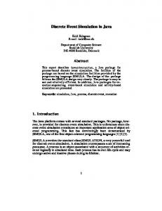
L’Ecuyer and Buist Table 1: Performance Comparison for EventDriven and Process-Driven Simulation: CPU Times (in seconds) to Simulate 105 Customers µ Queue Events Threads DSOL 2.0 0.50 0.11 1.29 73.5 1.8 0.71 0.12 1.31 75.8 1.6 1.09 0.12 1.37 77.6 1.4 1.77 0.12 1.43 80.5 1.2 4.04 0.11 1.54 85.6 1.0 272 0.11 4.44 101.8 0.8 10037 0.36 — 82.8 0.6 20059 0.34 — 64.8

is taken from DSOL (Jacobs and Verbraeck 2004). Unfortunately, none of them is fully satisfactory. Java threads are designed for real parallelism, not for the kind of simulated parallelism required in process-oriented simulation. In the Java Development Kit (JDK) 1.3.1 and earlier, green threads supporting simulated parallelism were available and our original implementation of processes described in L’Ecuyer, Meliani, and Vaucher (2002) was based on them. But green threads are no longer supported in recent Java runtime environments. The threads are true threads from the operating system. This adds significant overhead and prevents the use of a very large number of processes in the simulation. This implementation of processes with threads can be used safely only with the JDK version 1.3.1 or earlier. The second implementation, provided to us by Peter Jacobs, stays away from threads. It uses a Java reflexion mechanism that interprets the code of processes at run time and transforms everything into events. The implementation details are completely transparent to the user. There is no need to change the Java simulation program in any way, except for the import statement at the beginning of the program that decides which subpackage of simprocs we want to use. To demonstrate the loss of performance incurred when using processes instead of events, we report on the timing of a simulation of an M/M/1 queue using events and processes. Customers arrive according to a Poisson process with rate λ = 1 and have exponential service times with mean 1/µ. When a customer arrives while the server is busy, it is put in a FIFO queue with unlimited capacity. In an eventdriven simulation, each arrival and departure correspond to an event, and the waiting queue is represented by a list. In a process-driven simulation, each customer is represented by a process. The programs we used are very similar to those given in L’Ecuyer, Meliani, and Vaucher (2002). Table 1 gives the CPU times, in seconds, to simulate the system for 105 time units (approximately 105 arrivals), for different values of µ and with three different implementations: with events (Events), processes implemented by Java threads (Threads), and the DSOL implementation of processes (DSOL). The column marked Queue reports the average queue size, to give an idea of the number of simultaneous processes. For µ ≤ 1, the queue is unstable so the queue size increases steadily with the simulation length. This permits us to examine the effect of a large number of simultaneous processes on the performance, for process-driven simulation. These times were obtained with an AMD Athlon processor running at 2.088GHz, with Java Runtime Environment (JRE) 1.5 running under Linux. We see that the process-driven simulations are much slower than their event-driven counterparts, roughly by a factor of 12 for Java threads and a factor of 700 for DSOL. A greater queue size requires more internal node objects to store queued customers in a linked list, adding work

for the virtual machine. This explains why CPU times for events increase when the system is unstable. With threadbased processes, the CPU times increase with the number of simultaneous processes. When that number is too large, the program eventually crashes (this is why no CPU time is reported), not because of insufficient memory but due to a limitation on the number of native threads that can be provided by the operating system. With the DSOL solution, the only limitation on the number of threads is memory size. As long as the queue is stable (µ > 1), the execution time increases slowly with the average queue size. When the queue is unstable, decreasing µ reduces the number of events (ends of service) that occur during a given time period and this reduces execution times. The cost of the interpretation dominates the cost of object creation. 3

EXAMPLE: AN ASIAN OPTION

We provide an elementary example that illustrates how to generate random numbers, exploit the multi-streams facilities, compute distribution functions, and collect elementary statistics with SSJ. In this example, we price an Asian option by simulation, using randomized quasi-Monte Carlo to reduce the variance. We also show how to estimate a sensitivity via finite differences with common random numbers. 3.1 The Model A geometric Brownian motion (GBM) {S(ζ ),ζ ≥ 0} satisfies S(ζ ) = S(0) exp (r − σ 2 /2)ζ + σ B(ζ ) where r is the risk-free appreciation rate, σ is the volatility parameter, and B is a standard Brownian motion, i.e., a process whose increments over disjoint intervals are independent normal random variables, with mean 0 and variance δ over an interval of length δ (see, e.g., Glasserman 2004). The GBM process is a popular model for the evolution in time of the market price of financial assets. A discretely-monitored

615

L’Ecuyer and Buist interval on v. We have Var[X] ≈ 61.4 for this standard MC method.

Asian option on the arithmetic average of a given asset has discounted payoff X = e−rT max[S¯ − K, 0]

(3)

3.3 Common Random Numbers

where K is a constant called the strike price and 1 S¯ = S(ζj ), s

We now illustrate how the streams of SSJ are convenient for comparing two different configurations of a given system with common random numbers (CRNs) (Law and Kelton 2000). Let X1 denote the payoff X for a given value of σ = σ1 and X2 the payoff when σ = σ1 + δ, for some small δ > 0, and suppose we want to estimate E[X2 − X1 ]. This is useful, e.g., for estimating the sensitivity of the option price with respect to the volatility parameter σ (Glasserman 2004). If X1 and X2 are simulated with independent random numbers (IRNs), we have Var[X2 − X1 ] = Var[X1 ] + Var[X2 ] ≈ 2Var[X1 ]. Simulating them with CRNs means using exactly the same uniforms at exactly the same place for both X1 and X2 , to make Cov[X1 , X2 ] > 0. The method compareWithCRN performs n pairs of simulation runs with CRNs, using one substream of the given stream for each pair of runs. For each pair, we first generate the sample path for the current process and store the payoff X1 . The stream is then reset to the start of its current substream so that it will generate exactly the same sequence of random numbers when we generate the sample path for the second process, p2. The difference X2 − X1 is given as an observation to the statistical collector statDiff. Then the stream is advanced to the start of its next substream, ready for the next pair of runs. Here the two processes make exactly s calls to the RNG for each run. In general, however, when comparing similar systems with CRNs, the number of calls to the RNG may be “random” and differ across systems. Even in that case, using the SSJ substreams as illustrated here ensures that the RNG starts at the same place for both systems and that the sequences of random numbers that are used do not overlap. For complex systems, different RandomStream objects can be used for different parts of the system (e.g., in a queueing network, perhaps one stream for the interarrival times and one stream for the service times at each service station) to maintain synchonization. Then, all streams must be reset to their appropriate substreams between the runs. For this particular example, CRNs could be implemented by saving in an array the standard normal random variates produced by NormalDist.inverseF01 (stream.nextDouble()) in generatePath and reusing them for the second process. This would be more efficient because there would be no need to generate the uniforms and invert the normal distribution twice. But for more complicated system, the random variates are often generated from different distributions across systems and/or it is typically very inconvenient to store the random variates

s

(4)

j =1

for some fixed observation times 0 < ζ1 < · · · < ζs = T . The value (or fair price) of the Asian option is v = E[X] where the expectation is taken under a so-called risk-neutral measure (Glasserman 2004). 3.2 Pricing by Monte Carlo This v can be estimated by simulation as follows. Generate s independent and identically distributed (i.i.d.) N (0, 1) random variables Z1 , . . . , Zs and put B(ζj ) = B(ζj −1 ) +  ζj − ζj −1 Zj , for j = 1, . . . , s, where B(ζ0 ) = ζ0 = 0. Then, S(ζj ) = S(0)e(r−σ /2)ζj +σ B(ζj ) for j = 1, . . . , s and the payoff can be computed via (3). This can be replicated n times, independently, and the option value is estimated by the average discounted payoff. The Java program of Figures 1 and 2 implements this. Due to space limitations, we do not provide the most general and reusable program; for example, in a good design, the option (payoff function) and the underlying stochastic process might be defined in separate classes, the statistical collectors might be external and passed as parameters to the methods, etc. We have also removed certain parts of the program, including the import statements and some uninteresting instructions in the constructor. The Asian constructor  precomputes the discount factor e−rT and the constants σ ζj − ζj −1 and (r − σ 2 /2)(ζj − ζj −1 ), that depend on the process parameters and observation times. The method generatePath generates the values of S(ζj ) at the observation times, whereas getPayoff returns the corresponding option payoff. The method simulateRuns performs n independent simulation runs using the given random number stream and puts the n observations of the net payoff in the statistical collector statValue. In the main method, we first specify the s = 10 observation times ζj = (110 + j )/365 for j = 1, . . . , s, and put them in the array zeta (of size s + 1) together with ζ0 = 0. We then construct an Asian object with parameters r = log 1.09, σ = 0.2, K = 100, S(0) = 100, s = 12, and the observation times contained in array zeta. We then perform 106 (one million) simulation runs, and print the results. This took approximately 6.6 seconds to run on a 2.088GHz computer, with JRE 1.5 running under Linux, and gave (5.848, 5.870) as 95% confidence 2

616

L’Ecuyer and Buist public class Asian { double strike; // Strike price. int s; // Number of observation times. double discount; // Discount factor exp(-r * zeta[t]). double[] muDelta; // Differences * (r - sigmaˆ2/2). double[] sigmaSqrtDelta; // Square roots of differences * sigma. double[] logS; // Log of the GBM process: logS[t] = log (S[t]). // The array zeta[0..s+1] must contain zeta[0]=0.0, plus the s observation times. public Asian (double r, double sigma, double strike, double s0, int s, double[] zeta) { ... } // Generates the process S. public void generatePath (RandomStream stream) { for (int j = 0; j < s; j++) logS[j+1] = logS[j] + muDelta[j] + sigmaSqrtDelta[j] * NormalDist.inverseF01 (stream.nextDouble()); } // Computes and returns the discounted option payoff. public double getPayoff () { double average = 0.0; // Average of the GBM process. for (int j = 1; j strike) return discount * (average - strike); else return 0.0; } // Performs n indep. runs using stream and collects statistics in statValue. public void simulateRuns (int n, RandomStream stream, Tally statValue) { statValue.init(); for (int i=0; i