in CMOS-MEMS [4] and the new sensor networking technology. [5]. Motivated by that trend, ..... has a microcomputer chip (R8C/16, Renesas Technology Corp.).
B4-4
PROCEEDINGS OF THE 24TH SENSOR SYMPOSIUM,2007.pp.423∼427
3D Shape Capture Sheet Based on Gravity and Geomagnetic Sensing Takayuki Hoshi* and Hiroyuki Shinoda* In this paper, we introduce a novel sensing device named “three-dimensional capture sheet (3DCS).” The cloth-like sheet measures its own 3D configuration with no external equipments. It has many potential applications such as 3D modeling, entertainment, size and shape measuring, wearable motion capture, tactile sensor, and so on. It consists of a lattice structure inside of the sheet, and each link of the structure has a sensor chip consisting of a triaxial accelerometer and a triaxial magnetometer. The sensor chip measures the gravity and the Earth’s magnetic field to obtain the link posture. After all the link postures are obtained, the whole shape of the sheet is reconstructed by combining them. The estimation error from disturbed magnetic data is corrected by utilizing a constraint originating from the lattice structure. Feasibility and stability of the shape estimation algorithm are confirmed through simulations, and the prototype of the sensor chip is presented. Keywords : Sensor network, 3-dimensional configuration, Flexible sensing device, Gravity, Earth’s magnetic field
1.
Introduction
Providing intelligent functions for fabrics has often been reported in the field of wearable computing [1]-[3]. In early studies, in order to realize functionality, several middle-sized sensors were attached on fabrics or clothes. Recently, it is getting easier to embed a large number of down-sized and low-cost sensors in elastic cloth-like materials, due to the recent advances in CMOS-MEMS [4] and the new sensor networking technology [5]. Motivated by that trend, we propose a novel cloth-like device that measures its own 3D shape and motion by utilizing a large number of sensors distributed on it. The device is named “3-dimensional capture sheet (3DCS).” One of the conventional methods for observing the cloth motion is to utilize optical methods like the optical 3D digitizers [6]. However, such methods are weak against the self-occluding situation. In addition, optical methods require external equipments such as cameras and light sources, which can be drawbacks in some applications. The 3DCS does not suffer from the self-occlusion problem and requires no external equipments. The 3DCS has several potential applications. First, the device can be used in measuring the shape of 3D objects. The shape and size of an object can be measured easily by wrapping it with the 3DCS. The human posture can also be measured by wearing it. Second, it is possible to make a soft tactile sensor [7] with the 3DCS by covering compressible materials such as urethane foams with it. If the deformation of the surface of the material is given, the number, shapes, and positions of contact objects can be estimated. In addition to those applications described above, it is also useful to capture the 3D shapes of clothes for 3D modeling applications. In this paper, we discuss one of the realization methods of the 3DCS. Fig. 1 shows the structure of the 3DCS. A cloth-like sheet has a lattice structure on it. A triaxial accelerometer and a triaxial
Figure 1. Illustration of the 3DCS.
magnetometer are attached on each link. They measure the gravity and the geomagnetic vectors. The posture of the link is calculated using the measured data. After the postures of all the links are obtained, the whole shape of the sheet is computed by combining the links. That reconstruction algorithm is free from the well-known error accumulation caused by the double integration of the acceleration. Besides, both of the gravity and the Earth’s magnetic field are available everywhere on the Earth. In the previous reports [7], [8], we proposed the gravity-based method of the 3DCS. Although it works well in many cases, it has some singular states where reconstruction is impossible. We therefore propose a reinforced method by introducing the Earth’s magnetic field as additional information. Gravity and geomagnetic measurement has been used in motion capture in the preceding reports [9], [10]. We apply this technique to the 3DCS. The following paper describes the basic structure and the theory of 3D shape reconstruction of the 3DCS in Section 2. Feasibility of the sheet is examined by simulation in Section 3. Then, the current status of implementation is presented in Section 4. Then, Section 5 concludes the paper.
* Department of Information Physics and Computing, Graduate School of Information Physics and Technology, The University of Tokyo, 7-3-1 Hongo, Bunkyo-ku, Tokyo, Japan 113-8656
423
(a)
(b) Figure 3. World coordinate and posture angles.
the whole shape of the 3DCS is calculated by combining the links in a 3D space. The angles of the link are obtained as follows. Here we assume that each axis of the accelerometer and the magnetometer is aligned to the corresponding axis of the world coordinate (i.e. the x-axis of the accelerometer to the x-axis of the world coordinate) in the initial condition. 2.3 Derivation of Link Posture All the posture angles are derived directly from the gravity and the geomagnetic vectors measured with the sensor chip on each link. The rotation matrix Gγβα, from the world coordinate to the sensor coordinate, is described as
(c) Figure 2. (a) Lattice model made of rigid tubes combined with strings (7×7 lattice consisting of 2.5 cm links). (b) The lattice can be mounted on a smooth curved surface. For example, here it covers the ball. (c) The omni-directional lattice structure.
2.
Three-Dimensional Capture Sheet
2.1 Structure The illustration of the 3DCS is shown in Fig. 1. The 3DCS consists of rigid links forming a lattice structure. A sensor chip is attached on each link which has a triaxial accelerometer and a triaxial magnetometer. The accelerometer and the magnetometer measure the gravity and the geomagnetic vectors, respectively. The measured data are sent to the host computer. The x- and z-axes of both sensors are aligned to be parallel to the direction vector of the link. The length of each link is the same. The links are connected to each other at joints and rotate freely around the joints. Fig. 2 shows a mock-up of the 3DCS consisting of rigid tubes combined together using strings. Since the length of the link does not change, the lattice structure expands or contracts along the diagonal directions, as is the case with a textile cloth. As shown in Fig. 2 (b), the structure is able to cover a smooth curved surface. It is possible to make the lattice structure omni-directional by connecting the links little more intricately as shown in Fig. 2 (c). 2.2 Problem Settings First, we introduce an assumption to restrict the problem to a static case. The acceleration caused by motion of the link is negligible compared with the gravity acceleration. The shape estimation in a dynamic case is not considered at least in this stage. The 3DCS utilizes the gravity vector g and the Earth’s magnetic field b to estimate its configuration. We assume b is perpendicular to g, tentatively here. The real situation where b has a parallel component to g is mentioned in the end of Section 2.3. The world coordinate is set so that the z- and x-axes are parallel to g and b, respectively (Fig. 3). The posture of each link is described by three angles based on the world coordinate (Fig. 3); roll α [rad], pitch β [rad], and yaw γ [rad] (–π ≤ α < π, –π/2 ≤ β ≤ π/2, and 0 ≤ γ < 2π). The angles of each link are calculated from the measured gravity and geomagnetic vectors. After the angles of all the links are obtained,
G γβα
0 cγ − sγ 0 cβ 0 sβ 1 0 ≡ sγ cγ 0 0 1 0 0 cα − sα 0 0 1 − sβ 0 cβ 0 sα cα cγ cβ cγ sβ sα − sγ cα cγ sβ cα + sγ sα = sγ cβ sγ sβ sα + cγ cα sγ sβ cα − cγ sα ··· (1) − sβ cβ sα cβ cα
where “s” and “c” stand for “sin” and “cos”, respectively. Each column of Gγβα means the axis of the sensor coordinate represented in the world coordinate after rotated. The output vector of the accelerometer a = [ax, ay, az]T is represented as a product of the transposed matrix of Gγβα and the gravity vector g = [0, 0, -g]T (where g [m/s2] is the gravity acceleration);
a=G
T γβα
sβ . ················································· (2) g = g − cβ sα − cβ cα
Similarly, the output of the magnetometer m = [mx, my, mz]T is represented as a product of the transposed matrix of Gγβα and the geomagnetic vector b = [b, 0, 0]T (where b [T] is the flux density of the Earth’s magnetic field);
m=G
T γβα
cγ sβ . ··································· (3) b = b cγ sβ sα − sγ cα cγ sβ cα + sγ sα
Then α, β, and γ are obtained by solving (2) and (3) without knowledge of the values of g and b. After the same algorithm is applied to each link to obtain the roll, pitch and yaw angles, the whole configuration is estimated by combining them.
424
Figure 4. Lattice unit. Directional vectors form a closed-loop.
Figure 6. Simulation results for a Gaussian shape. The far and the near plots are the lattice model and the estimated shape, respectively.
3.
Figure 5. (a) Lattice unit in a disturbed magnetic field and (b) the estimated shape based on the parallel assumption. The dotted lines represent the magnetic field lines.
Simulations and Results
3.1 Methods The purpose of the simulation was to confirm if it was feasible to reconstruct the shape of a computational object based on the proposed algorithm. A computational model of a 13×13 lattice structure comprised of links was used as the model of the 3DCS. In this lattice model, the link was modeled as a rigid body so that the length of the link (2.0 cm) did not change, and the node was modeled as a free-joint. The lattice model was laid over a target computational shape. Position and posture of each link were determined by iterative calculation. According to the calculated postures of the links, the acceleration and the magnetic field vectors were simulated which were equivalent to the outputs of the accelerometers and the magnetometers. After that, based on the acquired acceleration and magnetic data, the shape of the computational object was estimated. The posture angles α, β, and γ were analytically determined by solving (2) and (3). In order to re-estimate the yaw angle γ, the following numerical calculation was conducted. First, we modify (5) into a minimization problem, that is
Note that the geomagnetic vector b makes the declination angle with the horizontal in the real situation, and hence the magnetometer output m has a parallel component to the accelerometer output a. A perpendicular component m' is used for the estimation algorithm instead of m, that is calculated as
a a . ···················································· (4) m' = m − m ⋅ | a | | a | The yaw angle γ can be obtained unless m' = 0 (which situation rarely occurs). The precise knowledge of the declination angle is not necessary. 2.4 Correction of Magnetic Disturbance The Earth’s magnetic field is easily disturbed by magnets, coils, or ferromagnetic materials. That leads to an estimation error on the yaw angle. We have an idea to correct this estimation error by utilizing a constraint originating from the lattice structure. Here we take note of one unit of the lattice structure composed of four links forming a quadrangle (Fig. 4). Because the directional vectors di (i is the link identification) of the links make a closed-loop; that is represented as
P≡
∑
( d 0 j + d 1 j − d 2 j − d 3 j ) 2 → min . ·················· (7)
j∈{ x , y , z }
where j is the coordinate identification. Here, γi are unknown parameters. If the minimum value of P is equal to zero, the solutions for (7) are also the solutions for (5). Second, we solve (7) by the conjugate gradient method [11]. The values of γi obtained from (3) are used as initial values. Accordingly, the probable values of γi are obtained. 3.2 Results of Shape Estimation An example of general situations using a Gaussian as a target shape is shown. Fig. 6 shows the computed lattice model laid over the Gaussian shape (plots at far side) and the reconstructed shape using the acceleration data (plots at near side). The Gaussian shape is successfully reproduced. 3.3 Effects of Acceleration and Magnetic Noises The results in Fig. 6 were obtained without considering the effects of noise. There are several possible causes of disturbance in the real situation, including random noise on the sensor data, change of the link length, and acceleration of motion. Among the causes listed above, the most major cause is considered to be the noise on the
d 0 + d 1 = d 3 + d 2 , ···························································· (5)
1 cγ i cβ i d i ≡ G γiβi α i 0 = sγ i cβ i . ············································ (6) 0 − sβ i When a magnetic disturbance occurs, the magnetic vectors at the sensor positions are no longer parallel (Fig. 5 (a)). Then the estimated shape based on the measured magnetic data results in an open-loop (Fig. 5 (b)). By solving (5) about γi around the values estimated from (3), γi are re-estimated so that the lattice unit becomes a closed-loop. This correction algorithm needs more mathematical analysis on solvability and uniqueness.
425
Figure 8. Simulation setting with a single-loop coil. The diameter is 10 cm and the current I is 10 A.
Figure 7. Simulation results on effect of noises. The worst cases of the maximum estimation error, i.e. the envelope of the error plot, are shown (10 trials per each noise level). The area where the maximum estimation error is lower than 15 % is colored deeply.
Figure 9. Simulation results on effectiveness of the correction algorithm. The horizontal axis is the distance d, normalized by the link length l, between the coil and the 3DCS.
(a) (b) Figure 7. Examples in the cases of (a) 5 % acc. and 20 % mag. noises, and (b) 10 % acc. and 20 % mag. noises.
acceleration data. In order to investigate the stability of the 3DCS under various S/N ratios, the following simulation was carried out. The simulation was carried out in the same manner as described in Section 3.1, except that noises were added to each component of the acceleration and magnetic data. The noises were generated using the Mersenne Twister algorithm [12]. The acceleration and magnetic noise levels were represented as the percentages of the noises compared to the gravity g and the geomagnetic flux density h, respectively. Fig. 7 shows the maximum values of the estimation errors as the function of the acceleration and magnetic noise levels. The estimation error of each trial is the maximum distance between the nodes of the lattice model and the corresponding nodes of the reconstructed model, which is normalized by the length of the side of the 3DCS. The reconstructed shape has uncertainty in the absolute position and posture. Therefore, the estimation errors were determined as follows. The sum of the distance between the nodes of the lattice model and the corresponding nodes of the reconstructed model (i.e. the estimation error sum) was calculated. The absolute position and posture of the reconstructed model were varied so that the estimation error sum was minimized based on the least-square method. Note that if no errors are added to the acceleration outputs, the lattice model and the reconstructed shape should be identical. 10 trials per each noise level were conducted. The maximum value of the estimation error among all the nodes was chosen and shown in Fig. 7 for each noise condition.
(a) (b) Figure 10. Examples in the cases with correction. (a) d/l = 0.9 (error = 1.1 %) and (b) d/l = 0.8 (error = 6.9 %).
From our observation of this simulation, it turned out that the maximum estimation error higher than 15 % (i.e. 39 mm) is critical. Based on that benchmark, it turns out that the noise levels are allowed up to 8 % for acceleration data (i.e. about 0.8 m/s2 in acceleration) and 25 % for magnetic data (i.e. about 7.5 µT in magnetic flux density in Tokyo). Typical examples are shown in Fig. 7; (a) successful and (b) unsuccessful. 3.4 Effectiveness of Correction Algorithm In order to examine effectiveness of the correction algorithm described in Section 2.3, the following simulation was carried out. It was carried out in the same manner as described in Section 3.1, except that a single-loop coil (magnetic source) added an additional magnetic field to the Earth’s magnetic field. The coil was parallel to the x-y plane and located just above the model shape at a distance d [m] from the surface of the 3DCS (Fig. 8). The
426
Acknowledgement This work is partly supported by JSPS Research Fellowships for Young Scientists. References (1)
IEEE International Symposium on Wearable Computers (ISWC ‘97), pp.
Figure 11. Hand-made trial circuit of the sensor chip (19×38 mm2). The chips mounted on the left and right sides are the microcomputer (6.4×6.5 mm2) and the 6-axis sensor (5.2×6.0 mm2), respectively.
167-168 (1997) (2)
IEEE International Symposium on Wearable Computers (ISWC ‘99), pp. 107-113 (1999) (3)
T. Linz, C. Kallmayer, R. Aschenbrenner, and H. Reichel, “Embroidering electrical interconnects with conductive yarn for the integration of flexible electronic modules into fabric,” Proc. 9th IEEE International Symposium on Wearable Computers (ISWC ‘05), pp. 86-91 (2005)
(4)
O. Brand, “Microsensor Integration into Systems-on-Chip,” Proc. IEEE, vol. 94, no. 6, pp. 1160-1176 (2006)
(5)
Y. Makino, H. Chigusa and H. Shinoda, “Two-dimensional sensor integration using resonant proximity connector -Basic technology and application to elastic interface device-,” Proc. 3rd International Conference on Networked Sensing Systems (INSS 2006), pp. 196-202 (2006)
(6)
M. Petrov, A. Talapov, T. Robertson, A. Lebedev, A. Zhilyaev, and L. Polonskiy, “Optical 3D digitizers: Bringing life to the virtual world,” IEEE Computer Graphics and Applications, vol. 18, pp. 28-37 (1998)
(7)
T. Hoshi and H. Shinoda, “Free-form tactile sensor using 3-dimensional shape capture sheet,” Proc. 2nd Joint Eurohaptics Conference and Symposium on Haptic Interfaces for Virtual Environment and Teleoperator
Implementation
Systems (World Haptics 2007), pp. 403-408 (2007) (8)
We are in the process of developing a prototype of the gravityand geomagnetic-based 3DCS. A small-sized sensor chip will be fabricated which has a 6-axis motion sensor (AMI601, Aichi Micro Intelligent Corp.). That sensor functions as both a 3-axis accelerometer and a 3-axis magnetometer. The sensor chip also has a microcomputer chip (R8C/16, Renesas Technology Corp.) which receives the measured data from the motion sensor and transmits the data to the host PC via an I2C bas line. Now it has been verified that the gravity and geomagnetic data are successfully obtained with a trial circuit of the sensor chip (Fig. 11). The next step is miniaturization and increase of production.
5.
J. Farringdon, A. J. Moore, N. Tilbury, J. Church, and P. D. Biemond, “Wearable sensor badge and sensor jacket for context awareness,” Proc. 3rd
diameter of the coil was 10 cm and the current I [A] was 10 A. The magnetic field arisen from the coil was calculated based on the Biot-Savart law. Fig. 9 shows the estimation errors as the function of the distances between the top of the model shape and the coil. The distance d is normalized by the link length l [m]. (Here, l = 2.0 cm.) Because this simulation was without random noises, 1 trial per each distance was conducted. From the results of the simulation, it turned out that the shape was successfully reconstructed even when the coil was located at a distance of 1.8 cm (d/l = 0.9) from the surface of the 3DCS. Then the estimation error was as small as 1.1 % (i.e. about 2.9 mm). The same error occurred when d = 9 cm (d/l = 4.5) in the case without correction. That suggests that the estimation algorithm works well unless magnetic sources or ferromagnetic materials come very close to or contact the 3DCS. Typical examples are shown in Fig. 10; (a) successful and (b) unsuccessful.
4.
E. R. Post and M. Orth, “Smart fabric, or “wearable clothing”,” Proc. 1st
T. Hoshi, S. Ozaki, and H. Shinoda, “Three-Dimensional Shape Capture Sheet Using Distributed Triaxial Accelerometers,” Proc. 4th International Conference on Networked Sensing Systems (INSS 2007), pp. 207-212 (2007)
(9)
J. Lee and I. Ha, “Real-time motion capture for a human body using accelerometers,” Robotica, vol. 19, pp. 601-610 (2001)
(10) D. Fontaine, D. David, Y. Caritu, “Sourceless human body motion capture,” Proc. Smart Objects Conference (SOC ‘03) (2003) (11) W. H. Press, S. A. Teukolsky, W. T. Vetterling, and B. P. Flannery, Numerical Recipes in C: The Art of Scientific Computing Second Edition, Cambridge University Press (1992) (12) M. Matsumoto and T. Nishimura, “Mersenne Twister: A 623-dimensionally
Conclusion
equidistributed uniform pseudorandom number generator,” ACM Trans. on Modeling and Computer Simulation, vol. 8, no. 1, pp.3-30 (1998)
This paper proposed a new flexible sensing device “3DCS,” which measures its own 3D configuration using distributed triaxial accelerometers and magnetometers. The details of the structure and the shape estimation algorithm were described. The feasibility of the algorithm was verified by simulation. Development of the prototype is in progress. In the future, we will develop a small-sized sensor chip on which a customized LSI is mounted with a triaxial accelerometer and a triaxial magnetometer. The LSI is designed to receive the sensor readouts and send digital data to the host computer via the two-dimensional communication sheet [5]. The required electrical power is also supplied via the same sheet to the sensor chips. Combining together with these technologies, the practical 3DCS will be realized without complicated long signal/power wires.
427