Three-Dimensional Shape Capture Sheet Using. Distributed Triaxial Accelerometers. Takayuki Hoshi, Sayo Ozaki, and Hiroyuki Shinoda. Department of ...
Proc. 4th International Conference on Networked Sensing Systems (INSS 2007), pp. 207-212, Braunschweig, (Germany), Jun., 2007.
Three-Dimensional Shape Capture Sheet Using Distributed Triaxial Accelerometers Takayuki Hoshi, Sayo Ozaki, and Hiroyuki Shinoda Department of Information Physics and Computing Graduate School of Information Science and Technology, The University of Tokyo Tokyo, Japan {star, ozaki, shino}@alab.t.u-tokyo.ac.jp
Abstract—In this paper, we propose a novel sensing device named “3-dimensional capture sheet (3DCS)”. The cloth-like sheet measures its own 3D configuration. It consists of a lattice structure inside of the sheet, and each link of the structure has a triaxial accelerometer. The roll and pitch angles of the link are calculated from the gravity vector measured with the accelerometer. Furthermore, the relative yaw angle is also determined by using constraints originating from the lattice structure. The whole shape of the sheet is reconstructed by combining the obtained postures of all the links. Keywords- sensor network; 3-dimensional configuration; flexible sensing device; triaxial accelerometer
I.
INTRODUCTION
Providing intelligent functions for fabrics has often been reported in the field of wearable computing [1]-[3]. In early studies, in order to realize functionality, several middle-sized sensors were attached on fabrics or clothes. Recently, it is getting easier to embed a large number of down-sized and low-cost sensors in elastic cloth-like materials, due to the recent advances in CMOS-MEMS [4] and the new sensor networking technology [5]. Motivated by that trend, we propose a novel cloth-like device that measures its own 3D shape and motion by utilizing a large number of sensors distributed on it. The device is named “3-dimensional capture sheet (3DCS)”. One of the conventional methods for observing the cloth motion is to utilize optical methods like the optical 3D digitizers [6]. However, such methods are weak for the self-occluding situation. In addition, optical methods require external equipment such as cameras and light sources, which can be drawbacks in some applications. The 3DCS does not suffer from the self-occlusion problem and requires no external equipment. The 3DCS has several potential applications. First, the device can be used in measuring the shape of 3D objects. The shape and size of an object can be measured easily by wrapping it with the 3DCS. The human posture can also be measured by wearing it. Second, it is possible to make a soft tactile sensor [7] with the 3DCS by covering compressible materials such as urethane foams with it. If the deformation of the surface of the material is given, the number, shapes, positions of the contact objects can be estimated. Furthermore, even the contact force can be measured if the Young’s
Figure 1. Illustration of 3DCS.
modulus of the material is known. In addition to those applications described above, it is also useful to capture the 3D shapes of clothes for 3D modeling applications. In this paper, we discuss one of the realization methods of the 3DCS. Fig. 1 shows the structure of the 3DCS. A clothlike sheet has a lattice structure on it. A triaxial accelerometer is attached on each link, and measures the gravity vector. The posture of the link is calculated using the measured gravity. After the postures of all the links are obtained, the whole shape of the sheet is computed by combining the links. This gravity-based method has the following merits. First, unlike the magnetic or electrical field, the gravity is not disturbed by the circumstances. Second, since our method does not integrate the acceleration to obtain the position, the 3DCS is free from the well-known error accumulation caused by the double integration of the acceleration. The gravity measurement has been used in the motion capture in the preceding reports [8], [9]. They used the gravity to obtain only the roll and pitch angles of a human arm. The output of a single triaxial accelerometer contains only the information about the two angles. They used other types of sensors such as an electromagnetic compass or a gyro sensor to acquire the yaw angle. Unlike them, we used multi accelerometers to estimate the yaw angles without any other kinds of sensors.
(a)
(b)
Figure 2. (a) Lattice model made of rigid tubes combined with strings (7×7 lattice consisting of 2.5 cm links). (b) The lattice can be mounted on a smooth curved surface. For example, it covers the ball as in this figure.
Figure 3. Definition of the rotational angles. α, β, and γ are the roll, pitch, and yaw angles, respectively. The orthogonal coordinate in this figure means the world coordinate.
The following paper outlines first, a description of the basic structure and the theory of 3D shape reconstruction of the 3DCS. Second, the feasibility of the sheet is examined by simulation in Section III. Then, the prototype is presented in Section IV. II.
THREE-DIMENSIONAL CAPTURE SHEET
A. Structure The illustration of the 3DCS is shown in Fig. 1. The 3DCS consists of rigid links forming a lattice structure. A triaxial accelerometer is attached on each link. The accelerometer measures the gravity vector and the measured data are sent to the host computer. The x- and z-axes of the triaxial accelerometer are aligned to be parallel to the direction of the link and to the direction of the normal vector to the sheet, respectively. The length of each link is the same. Fig. 2 shows a mock-up of the 3DCS consisting of rigid tubes combined together using strings. Since the length of the link does not change, the lattice structure expands or contracts along the diagonal directions, as is the case with a textile cloth. As shown in Fig. 2 (b), the structure is able to cover a smooth curved surface. B. Shape Estimation Algorithm First, we introduce the following assumption to restrict the problem to the static case. The shape estimation in dynamic motion is not considered at least in this stage. [Assumption 1] The acceleration caused by the motion of the link is negligible compared with the gravity acceleration.
Figure 4. Side view of the link. The sensor coordinate is rotated according to the roll and pitch angles, α and β.
The 3DCS utilizes the gravity vector measured with the accelerometer attached on each link to estimate its configuration. The posture of each link is described by three angles based on the world coordinate; roll α [rad], pitch β [rad], and yaw γ [rad] (Fig. 3). Though the roll and pitch angles of each link are calculated from the measured gravity vector, in order to estimate the relative yaw angle, constraints originating from the lattice structure are required. After the angles of all the links are obtained, the whole shape of the 3DCS is calculated by combining the links in a computational 3D space. Note that the estimated shape still has the uncertainty of orientation in the world coordinate. The details of the algorithm are discussed below. The angles of the link are obtained as follows. Here we assume that each axis of the triaxial accelerometer is aligned to the corresponding axis of the world coordinate (i.e. the xaxis of the accelerometer to the x-axis of the world coordinate) at the initial condition. 1) Roll and Pitch Angles: These angles are derived directly from the gravity vector measured with the accelerometer on each link. The rotation matrix Gβα, from the world coordinate to the sensor coordinate (Fig. 4), is described as
G βα
0 0 cos β 0 sin β 1 ≡ 0 1 0 0 cos α − sin α − sin β 0 cos β 0 sin α cos α cos β sin β sin α sin β cos α = 0 cos α − sin α . − sin β cos β sin α cos β cos α
(1)
Each column of Gβα means the axis of the sensor coordinate represented in the world coordinate after rotated, and hence the output vector of the accelerometer s = [sx, sy, sz]T is represented as a product of the transposed matrix of Gβα and the gravity vector g = [0, 0, -g]T (where g [m/s2] is the gravity acceleration);
g sin β s = G g = − g cos β sin α . − g cos β cos α T βα
Then α and β are obtained by solving (2).
(2)
Figure 5. Assumption 2. Since the lattice unit is a closed loop, the sum of the directional vectors d0+d1 is equal to d3+d2.
Figure 7. The shape of the lattice and the related angles used in the analysis on the unsolvability. The corner, fold, roll, and pitch angles were varied. Each angle was divided into 20 discrete values at even intervals.
[Assumption 3]
Figure 6. Assumption 3. We assume two types of symmetric transformations, (a) squashing and (b) folding. In such cases, the sum of the normal vectors n0+n2 is equal to n1+n3.
2) Yaw Angle: This angle cannot be calculated from the output of the single accelerometer. Therefore we made two assumptions, taking note of one unit of the lattice structure composed of four links forming a quadrangle. The first assumption is about the directional vector di (i is the link identification) which is represented as
cos γ i d i ≡ sin γ i 0
− sin γ i cos γ i 0
0 1 cos γ i cos β i 0 G βi α i 0 = sin γ i cos β i . (3) 0 − sin β i 1
n 0 + n 2 = n1 + n 3 .
(6)
γi is obtained by solving (4) and (6). Note that at least one of γi should be fixed to a certain value or given because this problem is underdetermined for all the four parameters γi in principle. Therefore the obtained yaw angels are relative solutions. Estimating the configuration of the multi-unit lattice structure is straightforward. After the same algorithm is applied to each lattice unit to obtain the roll, pitch and yaw angles, the whole configuration is estimated by combining the estimated unit shapes. C. Unsolvability Analysis The unsolvable conditions of (4) and (6) are clarified by the singular value decomposition (SVD) [10]. Now (4) and (6) are rewritten as a matrix form, that is,
Since the lattice unit is a closed loop (Fig. 5), the two routes reach the same point in the 3D space. That results in the Assumption 2, [Assumption 2]
d 0 + d1 = d 3 + d 2 .
(4)
The other assumption is about the normal vector ni which is represented as
cos γ i n i ≡ sin γ i 0
− sin γ i cos γ i 0
0 0 0 G β i α i 0 1 1
cos γ i sin β i cos α i + sin γ i sin α i = sin γ i sin β i cos α i − cos γ i sin α i . (5) cos β i cos α i We assume that the 3DCS is mounted on a smooth curved shape and the lattice unit transforms only in symmetric manners as shown in Fig. 6. In such case, the sum of one pair of the normal vectors of the opposite sides (in Fig. 6, n0 and n2, for example) must be equal to that of the other pair (n1 and n3). Hence,
(7) where “s” and “c” stand for “sin” and “cos”, respectively. The z-components of (4) and (6) are excluded because they do not contain any γi. Here γ0 is a fixed number to be the root of the orientation, and the other γi (i=1, 2, 3) are obtained as relative values to γ0. If the 4×6 coefficient matrix has less than three nonzero singular values, γi in (7) are underdetermined and the configuration of the lattice unit cannot be estimated uniquely. A model set of the lattice unit is generated by changing four angle parameters; corner θc [rad], fold θf [rad], roll θr [rad], and pitch θp [rad] (Fig. 7). Each angle is divided into 20 discrete values at even intervals. Fig. 8 reveals the unsolvable situations of (θc, θf, θr, θp). The points plotted in Fig. 8 stand for the conditions in which the ratio of the third singular value λ3 to the first largest singular value λ1 is less than 0.1 (i.e. λ3/λ1 < 0.1).
Figure 9. Simulation results for a Gaussian shape. The far and near plots are the lattice model and the reconstructed shape, respectively.
From Fig. 8, it turns out that most of the unsolvable conditions are roughly included in the following two cases: 1)
2)
All the links of the lattice unit are laid on a horizontal plane, i.e. (θf, θr, θp) = (0, 0, 0), (0, π, 0), (π, 0, 0), or (π, π, 0). The lattice unit is fully squashed, i.e. θc = 0, π, or θf = π.
Note that Case 2) is avoidable by setting limits to the range of angles of the link joints. Consequently, the essential unsolvable condition is only Case 1). III.
SIMULATIONS AND RESULTS
A. Methods The purpose of the simulation was to confirm if it was feasible to reconstruct the shape of computational objects based on the proposed algorithm. A computational model of a 13×13 lattice structure comprised of links was used as the model of 3DCS. In this lattice model, the links were modeled as very hard spring so that the length of the link did not change, and the nodes were modeled as mass. The lattice model was laid over a target computational shape and the position and posture of each link was determined by iterative calculation. According to the calculated postures of the links, the acceleration vectors which were equivalent to the outputs of the accelerometer were acquired. After that, based on the acquired acceleration vectors, the shape of the computational object was estimated. The roll and pitch angles were analytically determined using (2). On the contrary, it is hard to analytically obtain the yaw angles using (4) and (6). Therefore the following numerical calculation was conducted. First, we modify (4) and (6) into a minimization problem, that is Figure 8. Results of the analysis on the unsolvability. The (θc, θf, θr, θp)s satisfying λ3/λ1 < 0.1 were plotted in the parameter space. (a), (b), (c), (d), and (e) are for θc = 0, 45, 90, 135, and 180 deg, respectively. The plotted point means that the parameter set at the point gives unsolvable condition. From these graphs we concluded that (7) is solvable except for the trivial cases.
P≡
∑ {(d
0j
+ d1 j − d 2 j − d 3 j ) 2
j∈{ x , y , z }
+ (n0 j − n1 j + n2 j − n3 j ) 2 } → min.
(8)
where j is the coordinate identification. Now, αi and βi are given. If the minimum value of P is equal to zero, the solutions for (8) are also the solutions for (4) and (6). Second,
Figure 12. Sensor chip (14×38 mm2). It measures the gravity vector and transmits the measured data to the host PC via an I2C bus line.
Figure 10. Simulation results on the effects of the noise. The maximum values of the estimation error are plotted (10 trials per each noise level).
Figure 13. Prototype of the 3DCS (60×60 cm2). The length of each link is 10 cm. 12 sensor chips were used. (a)
(b)
(c)
Figure 11. Examples of the reconstructed shapes in the cases of (a) 5 %, (b) 6 %, and (c) 50 % noises.
we solve (8) by the steepest descent method. Although (8) has several local minima, by trying multiple initial parameter values, it is possible to avoid them in most cases. B. Results on Shape Estimation First, an example of general situations using a Gaussian as a target shape is shown. Fig. 9 shows the computed lattice model laid over the Gaussian shape (plots at far side) and the reconstructed shape using the acceleration data (plots at near side). The Gaussian shape is successfully reproduced. C. Effects of Noise on Acceleration Data The results in Fig. 9 were obtained without considering the effects of noise. There are several possible causes of disturbance, including the noise on the acceleration data, the change of the link length, and the violation of the Assumption 3 represented as (6). Among the causes listed above, the most major cause is considered to be the noise on the acceleration data. In order to investigate the stability of the 3DCS under various S/N ratios, the following simulation was carried out.
the side of the 3DCS. The reconstructed shape has uncertainty in the absolute position and posture. Therefore, the estimation errors were determined as follows. The sum of the distance between the nodes of the lattice model and the corresponding nodes of the reconstructed model (i.e. the estimation error sum) was calculated. The absolute position and posture of the reconstructed model were varied so that the estimation error sum was minimized based on the least-square method. Note that if no errors are added to the acceleration outputs, the lattice model and the reconstructed shape should be identical. 10 trials per each noise level were conducted. The maximum value of the estimation error among all the nodes was chosen and plotted in Fig. 10 for each trial. From our observation, it turned out that the 3DCS works under the condition that the noise level is up to 5 % (i.e. about 0.5 m/s2 in acceleration). It is possible to achieve this noise level when the actual 3DCS is fabricated. A critical estimation error such as Fig. 11 (b) or (c) frequently occurred when the noise level was higher than 6 %. IV.
PROTOTYPE
The simulation was carried out in the same manner as described in Section III A, except that the noise was added to each component of the acceleration data. The noise was generated using the Mersenne Twister algorithm [11]. The noise level was represented as the percentage of the noise compared to the gravity g.
A. System Specifications The integrated sensor chip was developed (Fig. 12). It consists of a triaxial accelerometer (AGS61231, Matsushita Electric Works, Ltd.) and a microcomputer (R8C/16, Renesas Technology Corp.). The analog outputs of the accelerometer are measured by the microcomputer using its 10-bit A/D converter. The microcomputer also transmits the measured data to the host PC via an I2C bus line.
Fig. 10 shows the maximum values of the estimation errors; the maximum distance between the nodes of the lattice model and the corresponding nodes of the reconstructed model. The estimation errors are normalized by the length of
Fig. 13 shows the prototype of the 3DCS. The side length of the sheet and each link are 60 cm and 10 cm, respectively. There are 12 sensor chips on the center, and they form a 2×2 lattice structure. The effective sampling rate of the system is
V.
Figure 14. Demonstration I: Flat plate.
CONCLUSION
This paper proposed a new flexible sensing device “3DCS”, which measures its own 3D configuration using distributed triaxial accelerometers. The details of the structure and the shape estimation algorithm are described. It is shown that the proposed estimation algorithm works well except for the trivial cases. The 2×2 prototype succeeded in estimating the shapes of a flat plate and a sphere with 7 % estimation error. We are working on developing the small-sized sensor chip on which an LSI is mounted with a triaxial accelerometer. The LSI is designed to measure the sensor readouts by A/D converters and send digital data to the host computer via the two-dimensional communication sheet [5]. The required electrical power is also supplied via the same sheet to the sensor chips. Combining together with these technologies, the practical 3DCS will be realized without complicated and long signal/power wires. REFERENCES [1]
Figure 15. Demonstration II: Sphere.
58 Hz. The conjugate gradient method [10] is applied in the estimation process for real-time performance. B. Demonstration I: Flat Plate Fig. 14 shows the shape estimation of a flat plate. The 2×2 lattice structure was successfully reconstructed in real-time. The slope error of the plate was 4.5 deg and the position error of the nodes is 7 % (i.e. 14 mm in length for 20-cm side length). These errors were caused by the alignment error of the accelerometer, the characteristics of the joint, and the computational error in the estimation process. C. Demonstration II: Sphere Fig. 15 shows the shape estimation of a sphere (23.2 cm in diameter). The lattice structure is also estimated successfully in this case.
E. R. Post and M. Orth, “Smart fabric, or “wearable clothing”,” Proc. 1st IEEE International Symposium on Wearable Computers (ISWC ’97), pp. 167-168, 1997. [2] J. Farringdon, A. J. Moore, N. Tilbury, J. Church, and P. D. Biemond, “Wearable sensor badge and sensor jacket for context awareness,” Proc. 3rd IEEE International Symposium on Wearable Computers (ISWC ’99), pp. 107-113, 1999. [3] T. Linz, C. Kallmayer, R. Aschenbrenner, and H. Reichel, “Embroidering electrical interconnects with conductive yarn for the integration of flexible electronic modules into fabric,” Proc. 9th IEEE International Symposium on Wearable Computers (ISWC ’05), pp. 8691, 2005. [4] O. Brand, “Microsensor Integration into Systems-on-Chip,” Proc. IEEE, vol. 94, no. 6, pp. 1160-1176, 2006. [5] Y. Makino, H. Chigusa and H. Shinoda, “Two-dimensional sensor integration using resonant proximity connector -Basic technology and application to elastic interface device-,” Proc. 3rd International Conference on Networked Sensing Systems (INSS 2006), pp. 196-202, 2006. [6] M. Petrov, A. Talapov, T. Robertson, A. Lebedev, A. Zhilyaev, and L. Polonskiy, “Optical 3D digitizers: Bringing life to the virtual world,” IEEE Computer Graphics and Applications, vol. 18, pp. 28-37, 1998. [7] T. Hoshi and H. Shinoda, “Free-form tactile sensor using 3dimensional shape capture sheet,” Proc. 2nd Joint Eurohaptics Conference and Symposium on Haptic Interfaces for Virtual Environment and Teleoperator Systems (World Haptics 2007), pp. 403-408, 2007. [8] J. Lee and I. Ha, “Real-time motion capture for a human body using accelerometers,” Robotica, vol. 19, pp. 601-610, 2001. [9] N. Miller, O. C. Jenkins, M. Kallmann, and M. J. Mataric, “Motion capture from inertial sensing for untethered humanoid teleoperation,” Proc. 4th IEEE/RAS International Conference on Humanoid Robots (Humanoids 2004), vol. 2, pp. 547-565, 2004. [10] W. H. Press, S. A. Teukolsky, W. T. Vetterling, and B. P. Flannery, Numerical Recipes in C: The Art of Scientific Computing Second Edition, Cambridge University Press, 1992. [11] M. Matsumoto and T. Nishimura, “Mersenne Twister: A 623dimensionally equidistributed uniform pseudorandom number generator,” ACM Trans. on Modeling and Computer Simulation, vol. 8, no. 1, pp.3-30, 1998.