second row: sample 14 (roofing shingle), sample 16 (cork), sample 18 (rug-a), sample 20 (styrofoam), sample 22 (lambswool); third row: sample 25 (quarry tile), ...
To appear in International Journal of Computer Vision, Vol. 59: No. 1, August 2004
3D Texture Recognition Using Bidirectional Feature Histograms Oana G. Cula Kristin J. Dana CS Department ECE Department Rutgers University Piscataway, NJ 08854 oanacula,kdana @caip.rutgers.edu �
Abstract Textured surfaces are an inherent constituent of the natural surroundings, therefore efficient realworld applications of computer vision algorithms require precise surface descriptors. Often textured surfaces present not only variations of color or reflectance, but also local height variations. This type of surface is referred to as a 3D texture. As the lighting and viewing conditions are varied, effects such as shadowing, foreshortening and occlusions, give rise to significant changes in texture appearance. Accounting for the variation of texture appearance due to changes in imaging parameters is a key issue in developing accurate 3D texture models. The bidirectional texture function (BTF) is observed image texture as a function of viewing and illumination directions. In this work, we construct a BTF-based surface model which captures the variation of the underlying statistical distribution of local structural image features, as the viewing and illumination conditions are changed. This 3D texture representation is called the bidirectional feature histogram (BFH). Based on the BFH, we design a 3D texture recognition method which employs the BFH as the surface model, and classifies surfaces based on a single novel texture image of unknown imaging parameters. Also, we develop a computational method for quantitatively evaluating the relative significance of texture images within the BTF. The performance of our methods is evaluated by employing over 6200 texture images corresponding to 40 real-world surface samples from the CUReT (Columbia-Utrecht reflectance and texture) database. Our experiments produce excellent classification results, which validate the strong descriptive properties of the BFH as a 3D texture representation.
Keywords: texture, 3D texture, bidirectional texture function, BTF, bidirectional feature histogram, BFH, appearance, appearance-based, recognition, texton, image texton.
1 Introduction The vast information embedded in visual imagery is organized at many levels: scenes are comprised of objects, objects are constructed from surfaces, and surfaces are described by reflectance and texture. Within this schematic of the visual world, surface descriptions form the foundation of image understanding. Indeed accurate surface models support appearance prediction which is central to many computer vision algorithms. 1
Figure 1: Several instances of the same crumpled paper sample, captured under different imaging conditions. The appearance changes significantly with variations in viewing and illumination directions. Descriptions of textured surfaces have suffered from oversimplification in much of the literature over the past couple of decades in computer vision. Texture viewed as a single image is a poor representation of the intricate interaction of light with real surfaces. Increasingly, recent work on texture representations deal with the complex changes of surface appearance with changes in illumination and viewing direction (Chantler, 1995) (Koenderink et al., 1999) (Leung and Malik, 1999) (van Ginneken et al., 1998) (Suen and Healey, 1998) (Dana and Nayar, 1998) (Dana and Nayar, 1999b) (Dana and Nayar, 1999a) (Suen and Healey, 2000) (McGunnigle and Chantler, 2000) (Cula and Dana, 2001b) (Cula and Dana, 2001a) (Liu et al., 2001) (Cula and Dana, 2002) (Tong et al., 2002) (Cula et al., 2003). Terminology for texture that depends on imaging parameters was introduced in (Dana et al., 1997) (Dana et al., 1999). Specifically, the term bidirectional texture function (BTF) is used to describe image texture as a function of the four imaging angles (viewing and light directions). The BTF can be interpreted as a spatially varying bidirectional reflectance distribution function (BRDF). The BRDF is defined as the the radiance reflected from a scene point divided by the irradiance and can be written as
������� � ��� �� �� �
��
illumination direction, respectively, and
�� �� �
where
����� � �
are the polar and azimuthal angles of the
are the polar and azimuthal angles of the viewing direction.
The dependence of on two directions is the reason this reflectance function is bidirectional. Models of the BRDF can be quite complex in order to capture the large variation of surfaces in real world scenes. But for a textured surface, reflectance also varies spatially. To capture this additional dimension, accurate models are needed for the BTF (bidirectional texture function) which can be written as �����
��������� ����� � ��� �� �� �
��
where
are Cartesian coordinates on the surface. To underscore the importance of accounting for variations with imaging parameters, consider Figure 1
which shows the same surface under different viewing and illumination directions. Clearly the “image texture” changes dramatically in this image set, while the underlying surface texture remains the same. It is tempting to use geometric models to describe 3D textured surfaces. While the surface texture often
2
exhibits fine scale geometry, the geometry is very difficult to model and sometimes impossible to measure. Even the most sophisticated laser range finders are poor at ascertaining very fine scale geometric changes. Furthermore, geometry is only part of the picture since the local reflectance is also quite important. Consider surface samples that exhibit 3D texture such as skin, orange peel, velvet, bark, linen, fur, etc. For these widely varying textured surfaces, no simple model can capture the rich variation in local reflection and the contribution of the fine scale geometry in an effective manner. These issues have led to the increasing popularity of exemplar-based or appearance-based approaches. Recent work in surface texture addresses the dependence of appearance on imaging conditions. The CUReT database (Dana et al., 1997) (Dana et al., 1999) provides a starting point in empirical studies of textured surface appearance and it has been used in numerous recent studies (Koenderink et al., 1999) (van Ginneken et al., 1998) (Leung and Malik, 1999) (Leung and Malik, 2001) (Suen and Healey, 1998) (Dana and Nayar, 1998) (Dana and Nayar, 1999b) (Dana and Nayar, 1999a) (Suen and Healey, 2000) (Liu et al., 2001) (Cula and Dana, 2001b) (Cula and Dana, 2001a) (Cula et al., 2003) (Varma and Zisserman, 2002). This database contains texture and reflectance measurements from over 60 different samples, each observed with over 200 different combinations of viewing and illumination directions. Methods for 3D texture recognition using appearance-based representations derived from these image sets are discussed in (Leung and Malik, 1999) (Suen and Healey, 1998) (Dana and Nayar, 1999a) (Varma and Zisserman, 2002) (Penirschke et al., 2002). In (Dana and Nayar, 1999a) the texture representation is the conditional histograms of the response to a small multiscale filter bank. Principal component analysis is performed on the histogram of filter outputs and recognition is done using the SLAM library (Nene et al., 1994) (Murase and Nayar, 1995). The preliminary recognition results in this experiment were encouraging and motivated the work presented in this paper. In (Suen and Healey, 1998) the individual texture images are represented using multiband correlation functions that consider both within and between color band correlations. Principal components analysis is used to reduce dimensionality of the representation and this color information is used to aid in recognition. However, the use of texture color in (Suen and Healey, 1998) greatly assists the recognition since many of the samples in the test dataset are well separated in color space. In (Leung and Malik, 1999) a 3D texton is created by using a multiscale filter bank applied to an image set for a particular sample. The filter responses as a function of viewing and illumination directions are clustered to form appearance features that are termed 3D textons. In this paper we refer to this method
3
as the 3D texton method. The methods of (Varma and Zisserman, 2002) and (Penirschke et al., 2002) are recent 3D texture recognition methods which have the property of rotation invariance. The classifier in (Penirschke et al., 2002) can classify textures imaged under unknown illumination angle. The methods of (Varma and Zisserman, 2002) are similar to that of (Cula and Dana, 2001a) because image features are defined and then the set of feature histograms are used to represent the texture. The image features in (Varma and Zisserman, 2002) are the maximal filter response over a set of orientations and therefore is a rotational invariant description. The classical standard framework for 2D texture representation consists of a primitive and a statistical distribution of this primitive over space. So the pertinent question is: how does one extend a standard texture representation to account for 3D texture, where image texture changes with imaging parameters? To accomplish this extension, either the primitive or the statistical distribution should be a function of the imaging parameters. Using this framework, the comparison of our approach with the 3D texton method is straightforward. The 3D texton method uses a primitive that is a function of imaging parameters, while our method uses a statistical distribution that is a function of imaging parameters. In our approach the histogram of features representing the texture appearance is called bidirectional because it is a function of viewing and illumination directions. We accomplish a similar goal to that of the 3D texton method, namely precise recognition of textured surfaces. However our approach uses less a priori information and a fundamentally simpler computational representation.
2 BTF-based 3D Texture Representation We design a 3D textured surface representation based on the BTF, which captures the complex dependency of the texture appearance on the imaging conditions. The proposed representation necessitates the creation of a reduced collection of representatives among the local structural features encountered within texture images. For each texture image in the BTF a feature histogram is computed to approximate the distribution of key features over the image. The surface descriptor is the collection of feature histograms corresponding to the set of texture images within the BTF. Due to the dependency of texture images on both illumination and viewing directions, our texture representation is referred to as a bidirectional feature histogram. The feature histogram space is highly dimensional and complex, thus dimensionality reduction is achieved by
4
Unregistered Images from Unknown View/ Illumination
}
F
*
Sample 1
F
* . .
.
.
.
.
F
q
*
Sample 2 . . . Sample Q
Texton Labels
K-Means Clustering on size f Feature Vectors
Figure 2: Creation of the image texton library. The set of unregistered texture images from the BTF of each of the samples are filtered with the filter bank consisting of filters, i.e. filters for each of the three scales. The filter responses for each pixel are concatenated over scale to form feature vectors of size . The feature space is clustered via k-means to determine the collection of key features, i.e the image texton library.
�
�
�����
�
�
employing principal component analysis (PCA). The resulting surface descriptor is a manifold in the reduced eigenspace, parameterized by the imaging parameters.
2.1 Textons and Image Texton Library Within a texture image there are certain canonical structures, i.e. short edges with different orientations and phases, or spot-like features of various sizes, therefore we seek a reduced set of local structural features. Early psychophysical studies brought evidence that discrimination of black and white textures is based on pre-attentively discriminable conspicuous local features called textons (Julesz, 1981). Based on the classic concept of textons, and also based on modern generalizations (Leung and Malik, 2001), we obtain a finite set of local structural features that can be found within a large collection of texture images from various samples. We follow the hypothesis that this finite set, called the image texton library, closely represents all possible local structures. Figure 2 schematically illustrates our approach for constructing the image texton library. A widely used computational approach for encoding the local structural attributes of textures is based on multichannel filtering (Bovik et al., 1990) (Jain et al., 1999) (Randen and Husoy, 1999) (Leung and Malik,
5
2001). To obtain a computational description of the local feature we employ a multiresolution filter bank with size denoted by
� � �
�
,
, and consisting of Gaussian filters and center surround derivatives of Gaussian
filters on three scales. Each pixel of a texture image is characterized by a set of three multi-dimensional feature vectors obtained by concatenating the corresponding filter responses over scale. For simplicity in our discussions we will refer to a single scale, but it is important to keep in mind that the processing is done in parallel for all three scales. As in many approaches in texture literature (Leung and Malik, 2001) (Aksoy and Haralick, 1999) (Puzicha et al., 1999) (Ma and Manjunath, 1996), we cluster the feature space to determine the set of prototypes among the population. Specifically, we invoke k-means algorithm, which is based on the first order statistics of the data, and finds a predefined number of centers in the data space, while guaranteeing that the sum of squared distances between the initial data points and the centers is minimized. The resulting image texton library is required to be generic enough to represent a large set of 3D texture samples, and comprehensive enough to allow discrimination among different 3D texture samples. In order to verify these two properties, we design two recognition experiments. In the first experiment we use the same 3D texture samples for creating the image texton library and for recognition. The second experiment uses two disjoint 3D texture sample sets for the construction of the image texton library and for recognition. The results are discussed in Section 5.
2.2 Texton Histograms The histogram of image textons is used to encode the global distribution of the local structural attribute over the texture image. This representation, denoted by
�
��� �
�
, is a discrete function of the labels induced by the
image texton library, and it is computed as described in Figure 3. Each texture image is filtered using the same filter bank
�
as the one used for creating the texton library. Each pixel within the texture image is rep-
resented by a multidimensional feature vector obtained by concatenating the corresponding filter responses over scale. In the feature space populated by both the feature vectors and the image textons, each feature vector is labeled by determining the closest image texton. The spatial distribution of the representative local structural features over the image is approximated by computing the texton histogram. Given the complex height variation of the 3D textured sample, the texture image is strongly influenced by both the viewing direction and the illumination direction under which the image is captured. Accordingly, the corresponding image texton histogram is a function of the imaging conditions.
6
Texton Labels
F Texture Image I1
*
Texton Labeling
Compute Texton Histogram
variation of imaging parameters
. . .
. . . Texton Labels
F
Texture Image I n
H1(l)
*
Texton Labeling
Hn(l)
Compute Texton Histogram
Bidirectional Feature Histogram (BFH) ������� � � �
�
Figure 3: 3D texture representation. Each texture image �� , is filtered with filter bank , and filter responses for each pixel are concatenated over scale to form feature vectors. The feature vectors are projected onto the space spanned by the elements of the image texton library, then labeled by determining the ��closest texton. The distributions of labels over the images are approximated by the texton histograms � � ��� ��� � � � � � . The set of texton histograms, as a function of the imaging parameters, forms the 3D texture representation, referred to as the bidirectional feature histogram (BFH). Note that in our approach, neither the image texton nor the texton histogram encode the change in local appearance of texture with the imaging conditions. These quantities are local to a single texture image. We represent the surface using a collection of image texton histograms, acquired as a function of viewing and illumination directions. This surface representation is described by the term bidirectional feature histogram. It is worthwhile to explicitly note the difference between the bidirectional feature histogram and the BTF. While the BTF is the set of measured images as a function of viewing and illumination, the bidirectional feature histogram is a representation of the BTF suitable for use in classification. Prior attempts that use histograms to capture the dependency of the texture appearance on the imaging conditions include (Dana and Nayar, 1998) (van Ginneken et al., 1999). In (Dana and Nayar, 1998), an analytical model for the bidirectional intensity histogram is formulated, while in (van Ginneken et al., 1999) texture histograms as a function of surface illumination and viewing directions are obtained using surface imaging simulations. However, it is unlikely that a single, concise, theoretical model can fully account for
7
Texton Labels
Texture Image I1
Texton Labeling
. . .
H1(l)
Compute Texton Histogram
variation of imaging parameters
. . . HN (l)
}
M (s) R
PCA Reference Manifold in Eigenspace
Texture Image I N
�� ��
BFH
� ��
Figure 4: The construction of the reference manifold . The bidirectional feature histogram (BFH) is ��� � � � � computed using all texture images � , available within the sampled BTF. PCA is employed to reduce the dimensionality, and the resulting representation in the eigenspace is the reference manifold � �� , indexed by both the viewing and the illumination directions.
�� ��
�
�
the varied appearance of real world surfaces. The bidirectional feature histogram provides an encompassing representation, but it requires exemplars for constructing the surface descriptor. The dimensionality of histogram space is given by the cardinality of the image texton library, which should be inclusive enough to represent a large range of textured surfaces. Therefore the histogram space is high dimensional, and a compression of this representation to a lower-dimensional one is suitable, providing that the statistical properties of the bidirectional feature histograms are still preserved. To accomplish dimensionality reduction we employ PCA, which finds an optimal new orthogonal basis in the space, while best describing the data. This approach has been inspired by (Murase and Nayar, 1995), where a similar problem is treated, specifically an object is represented by set of images taken from various poses, and PCA is used to obtain a compact lower-dimensional representation. By performing eigenanalysis in the texton histogram space, we did not impose any assumption of Lambertian reflectance of the surface. PCA is employed not directly on the reflectance values, but on the set of texton histograms, therefore our assumption is that the corresponding projected points in the lowerdimensional eigenspace still retain the descriptive properties of the original bidirectional feature histogram. Our experimental results support this assumption.
8
B 3 2.5 2
B
1.5 1 0.5
A
0 1
0.5
1 0.5
0 0
A
�
���
� �� � �
�
�
� �
Figure 5: The points in the 3D space of imaging angles: , , and . The endpoints are denoted by ’o’. The texture images corresponding to the endpoints points A and B of the manifold, are exemplified for sample 4 (rough plastic). The imaging conditions under which texture image A has been captured are � � � � �
� ��� � � � � , , , , while those under which texture image B has been � � � � � � � � � � � , , , . imaged are
��
�� �� � � �� ���� ����� �� �
�� ��� � ��� �� ��� �� ���� ��� �� �
2.3 Compact Representation of the BTF Let us consider that each BTF consists of When
�
�
texture images, each captured under certain imaging conditions.
is very large, as is the case with the CUReT database, where
�
= 205, the space of the imaging
conditions is densely sampled, giving rise to texture images which might present great similarities. We hypothesize that a subset of this comprehensive representation carries redundant information about the local structure of the surface. In other words, we assume that there exists a subset of texture images which is sufficient for characterizing the 3D textured sample. As discussed in Section 2.2, our proposed BTF-based texture representation is obtained by employing the set of texton histograms to determine the parametric eigenspace, onto which the bidirectional feature histogram is projected. The intuition is that there exists an intrinsic topology within the set of points in the eigenspace. That is, we assume that the projected points lie on a continuous manifold parameterized by the imag-
�
�� �
�
�
�� , i.e. the polar and azimuthal angles of viewing direction, and the polar and azimuthal angles
ing conditions. Let
denote this manifold, where parameter
� �� �
�� ����� � �
of illumination direction, respectively. 9
is indexed by the imaging parameters
}
M 1 (s) . . .
M i (s) . . .
MN-2 (s)
MR (s)
di Compute Distance to Reference Manifold
Ordinal Scale of Texture Image Significance within BTF
Distance Distribution
Reduced-by-one Manifolds
� ��
� � �
��
Figure 6: The second step involved in� computing the compact representation of the BTF. The set of distances � ��� � �� � � � � between the reference manifold and the set of reduced-by-one manifolds , is used to determine the order of significance of various texture images within the BTF. To identify the core subset of texture images for a certain textured surface we design a quantitative evaluation method for measuring the significance of individual texture images within the overall representation. The three main steps involved in determining the reduced representation of the BTF are depicted in Figures 4, 6 and 7.
� ��
First, as illustrated in Figure 4, we construct a comprehensive representation of the BTF, called the reference manifold
�
�
, which is based on all
�
texture images available for representing the surface. Ideally,
this surface appearance manifold is a hypersurface parameterized by four parameters:
��
,
���
,
�
and
� �
, i.e.
the reference manifold is a 4-dimensional surface embedded in the high dimensional eigenspace. In prac-
�
� . While constructing the
tice, for the sake of simplicity, we choose to reduce the 4-dimensional manifold to a one dimensional curve,
�
parameterized by , where
�
is indexed by the imaging parameters
� � � � � � � � �
� � . The use of the difference
reference manifold, a predefined ordering of the projected points is necessary. The ordering that we use is defined in the 3-dimensional space of imaging angles: in azimuthal angles
�
�
,
���
, and
instead of individual azimuthal angles
��
���
and
�
� �
� �
is strictly correct when the imaged
textured surface is isotropic. Because all surfaces employed in our experiments are approximately isotropic, �
for ordering purposes we employ . The diameter of the set of points in the 3D space of angles is determined. Then, starting from one of the diametral points, the manifold path is constructed by choosing at each
10
}
1
M (s) . . .
M i (s) . . . N-2
M (s)
MR (s)
d
τ
i
Compute Distance to Reference Manifold
α
M (s)
Thresholding
Distance Distribution
Compact Representation of BTF
Reduced-by-i Manifolds
� ��
� ���
��
� Figure 7: The last task employed during the creation of the compact representation� �of� the BTF. The distances � �� �� � � � � between the� � reference manifold and the reduced-bymanifolds are �� � � is obtained by eliminating from the� �subset of least significant texture images computed. � within the� �BTF. The compact representation of the BTF, , is the reduced manifold at distance � from , where is no larger than a threshold , defined in Equation 2.
� ��
��
�
� ��
�
�� ��
�
step the closest unassigned point. The metric employed is the Euclidean distance. There are two reasons for this ordering. First, we want the curve representing the manifold to have relatively small variations between two neighboring knot points. Second, we want to objectively compare from one sample to another how removal from the manifold of a point corresponding to a certain combination of imaging parameters affects the overall topology of the manifold. The second task involved in constructing the compact representation of the BTF is illustrated in Figure 6.
� �� �
�
� indexed from to � from
the point at position , where �
�
� � � � �
��
� � ��
� � � , given that the �
It consists of creating the set of reduced-by-one manifolds, denoted by �
, each obtained by removing points on the manifold are
. The manifold endpoints are not removed because they typically represent texture
� � � knot points. The set of �� �� and the reference � �� .
images captured under very distinct imaging conditions, as illustrated in Figure 5. Each of the resulting reduced-by-one manifolds analyzed to compute the set of distances
�
��
��� ��
between each
has
��� ��
�
��� ��
is further
�
In practice, each manifold is sampled at a very high rate, and it is stored as a list of points in a multidimensional space. We define the distance between two manifolds as the average of the set of point-to-point distances. Therefore, in order to compute a meaningful distance between two manifolds we need to sample
11
both manifolds at the same rate. Based on the distribution of distances and
� �� �
�
�
between
��
���
�
�
,
� � � � �
� � �, �
, we define an ordinal scale for the relative significance of individual texture images within the
BTF. The most important and least important images within the BTF are identified by considering how the manifold changes when the image is removed. The most important texture image is the one that when removed generates the largest distance
�
between
��
� � ��
least important image generates the smallest distance
�
and the reference
� �� �
�
. Similarly, removal of the
.
Note that the second step of the proposed algorithm, intended to determine an importance ordering for the texture images within the sampled BTF, necessitates a uniform or quasi-uniform distribution of the sampled points on the hemisphere of all possible imaging conditions. If this property is violated, e.g. the BTF is sampled multiple times at the same point or at very close points, then the algorithm is not accurate anymore, because the texture images corresponding to these points would all be labeled as insignificant.
��
One way to overcome this issue is to modify the current approach such that every time a point is eliminated ��� ��
from the manifold and the distance between the corresponding reduced-by-one manifold ����
reference
�
and the
is very reduced, then this point is permanently eliminated from the manifolds, including
the reference. However, this modified approach greatly affects the efficiency of the algorithm. The CUReT database is constructed such that the property of uniform sampling of the viewing and illumination directions over the hemisphere is ensured, therefore we take advantage of this property, and we utilize the initial approach. Another important property of the CUReT database is that the imaging conditions corresponding to the points in which the BTF is sampled, are known. This property allows us to impose the ordering of knot points on the manifold, which is required for objective comparison of the significance of various imaging parameters from one texture sample to another.
� ��� , as it is described in Figure 7. ��
The third step in constructing the compact representation of the BTF consists of creating the set of �
reduced-by- manifolds
�� �
�
,
�
� � � � � �
�
� ��
is obtained by
eliminating points from the manifold, these points being chosen in accordance with the order of signifi�
cance of individual texture images within the BTF. That is,
� ��
�� �
�
�
� � �
first least significant points are removed. The distribution of the distances between and
�
�
�
, denoted by
, is used in determining which of the
� ��
is defined as the manifold from which all
��
� ��
,
�
� � � � � �� �
reduced-by- manifolds
�� �
�
is suf-
ficiently representative, while still encoding the most significant local structural properties of the textured surface. The compact representation
� ��
� ��
is determined by imposing that its distance
12
�
to the reference
(a)
(b)
Figure 8: Two surface samples from the CUReT database: (a) felt and (b) painted spheres, illustrated by their most significant texture image within the BTF. Notice how well the surface structural detail is depicted in these images.
�
manifold should not be larger than a threshold . More specifically:
� �
�
�
���� ��� � � � � ��
�
�
�� �
where
�
���� ������ ���� �
�
and
����� �
�� � ��� � � � � �� �
�
� � �
(1)
�� � �
(2)
(3)
Consider the imaging parameters corresponding to the most important texture image within the BTF, as it is determined by our method. In our experiments we notice that these important imaging parameters vary from one surface to another, especially when the two surfaces have very distinct local structural features. However, for many samples the most significant texture image is a near frontal view with an oblique illumination that casts shadows and emphasizes structural detail. As an example, consider two surface samples from the CUReT database: felt (sample 1) and painted spheres (sample 35). The
�� � �
���
��� �����
, while the most significant texture image within the ')( �� �� ')( ��� *')( � � �� �� *')( . The
most significant texture image within the BTF for sample 1 is captured under the imaging parameters:
�!
�
�
�
"! �$# �
� �
%!
� ���
�
&!
�
�� � �
BTF of sample 35 has as imaging parameters:
��
�
� �
�� �
�
�
�� � �
�
� � �
�
most significant images of both samples are illustrated in Figure 8. Note how well the geometric detail is 13
Texton Labels
Sample 1 Texture Image I1
Compute Texton Histogram
Texton Labeling
. . .
H1(l)
variation of imaging parameters
. . .
Hp (l)
Texture Image Ip
BFH1
. . .
. . .
Texton Labels
Sample P
Texture Image Ip
.
variation of imaging parameters
M{P}(s)
. . . Hp (l)
.
. . .
M{1}(s)
.
Compute Texton Histogram
Texton Labeling
Texture Image I1
H1(l)
}
PCA
Universal Eigenspace
BFH P ���
�
� � � �
Figure 9: The training step of the image texton method. The set of texture images � , for each of the � samples, is processed to compute its corresponding BFH. In the space spanned by the set of BFH’s for all � surface samples, PCA is employed and the universal eigenspace is obtained. The projected points � � � corresponding to a certain 3D texture sample, say sample � , lie on a parametric manifold indexed by the imaging conditions.
� � ��
depicted in these images. In Section 5 we further discuss the implications of the complexity of fine scale geometry of surface upon the compact representation of the BTF.
3 Image Texton Recognition Method The 3D texture recognition method consists of three main tasks: (1) creation of image texton library, (2) training, and (3) classification. The image texton library is described in Section 2.1 and illustrated in Figure 2. To extract meaningful textural features we employ a multichannel filter bank images, for each of the
�
3D texture samples, is filtered by
�
�
. Each of the
texture
and the filter responses corresponding to a
pixel are concatenated to form the feature vector. The feature space is populated with the feature vectors from all
� ��
images. Considering that texture has repetitive spatial properties, and that different textures
exhibit similar local structural features, it is reasonable to assume that the data populating the feature space 14
Texton Labels
Novel Texture Image
Compute Texton Histogram
Texton Labeling
H(l)
Project to Universal Eigenspace
Find Nearest Manifold
Figure 10: The classification task of the image texton method. A novel texture image, captured under ��� � � ��� � � unknown imaging conditions, is processed to compute its texton histogram . is projected onto the universal eigenspace, and the closest point is found. The surface sample corresponding to the manifold onto which the closest point lies is the class of the query. is redundant. Feature grouping is performed via k-means algorithm, and the representatives among the population are found, forming the image texton library. During training, a 3D texture model for each of the 3D texture samples is constructed. Figure 9 illustrates the steps involved in this task. The subset of texture images used for training is arbitrarily sampled from the entire BTF, or it is carefully planned as we suggest in Section 2.3, i.e. the training set is constructed based on the compacted BTF for each surface sample. In our experiments, for comparison reasons, we design the training task in both ways. Each of the
texture images considered for each of the �
be classified, is filtered by the same filter bank
�
3D texture samples to
as the one involved for constructing the texton library. The
resulting multidimensional feature vectors, obtained by concatenating the filter responses for a certain pixel in the image, are labeled relative to the set the image textons. For each texture image a texton histogram is computed. Therefore each 3D texture sample is characterized by the set of
texture histograms, referred to
as a bidirectional feature histogram (BFH). The set of BFH’s corresponding to the set of 3D texture samples are employed to compute the universal eigenspace, where each 3D texture sample is modeled as a densely sampled manifold. In the classification stage, illustrated in Figure 10, the subset of testing texture images is disjoint from the subset used for training. Again, each image is filtered by
�
, the resulting feature vectors are projected in the
image texton space and labeled according to the texton library. The texton distribution over the texture image is approximated by the texton histogram. The classification is based on a single novel texture image, and it is accomplished by projecting the corresponding texton histogram onto the universal eigenspace created during training, and by determining the closest point in the eigenspace. The 3D texture sample corresponding to the manifold onto which the closest point lies is reported as the surface class of the testing texture image.
15
To demonstrate the versatility of the image texton library we design two classification experiments. The first experiment uses the same set of textured surfaces for all three tasks involved during the image texton recognition method, while the second experiment uses two disjoint sets of 3D texture samples, one employed in creating the image texton library, and the other involved for recognition. The results are discussed in Section 5.
4 Comparison with 3D Texton Recognition Method 4.1 Summary of 3D Texton Recognition Method While recognition of 2D textures has been treated extensively, 3D texture recognition has received limited attention. The most notable prior work is the 3D texton method (Leung and Malik, 1999) (Leung and Malik, 2001). For comparison reasons, we briefly summarize this method here. The approach defines and uses the notion of 3D texton, which essentially is a surface feature, parameterized by both viewing and illumination directions. The method consists of 3 main steps: (1) creation of the 3D texton vocabulary, (2) training, and (3) classification. During the first step, depicted in Figure 11(a), a collection of 3D textons is constructed by using
�
3D texture samples, each represented by
texture image is filtered by a multichannel filter bank a pixel, and corresponding to all
spatially aligned texture images. Each
�� , of size �� . The filter responses corresponding to
registered texture images of a certain BTF, are grouped together into a
highly dimensional feature vector of size
� �
. The resulting feature vector encodes the variations of local
structure at a pixel due to changes in the imaging conditions. Because of repetitiveness of local structures within textured surfaces, and to the local similarities between different textures, the set of spatial features is redundant, and it is compacted to a reduced set of prototypes, termed 3D textons. The set of 3D textons is obtained by performing k-means clustering in the highly dimensional feature space. The training stage is illustrated in Figure 11(b). It consists of creating the 3D texture models for all surfaces to be classified. Each 3D texture sample is represented by the 3D texton histogram obtained by first filtering registered texture images, captured under the same imaging conditions as the texture images used for creating the 3D texton vocabulary. Then the filter responses of a pixel are aggregated to form feature vectors, which are labeled according to the 3D texton vocabulary. The classification is performed with two methods. The first approach, shown in Figure 11(c), is non-iterative, and uses a set of novel registered
16
texture images for testing, with known imaging conditions. This set of texture images is processed to determine the corresponding 3D texton histogram, and classification is performed by computing the chisquare distance between all model histograms and the query. The texture class is determined by the closest model histogram. The second classification approach, summarized in Figure 11(d), is based on a single novel texture image with unknown imaging conditions, and uses an iterative Markov Chain Monte Carlo algorithm with Metropolis sampling to obtain texton labelings and a material classification.
4.2 Comparison of Methods Every appearance-based texture modeling technique must encode the global distribution of various local structural features over the texture. Furthermore, a suitable representation of 3D texture, presenting fine scale geometry, must also capture the variations of local appearance due to changes in imaging conditions. Both methods, the image texton method, as well as the 3D texton method, have texture representations which satisfy these requirements. However, there are fundamental differences. The primitive of the 3D texton method is the 3D texton, a salient local structural feature of a surface, as a function of the view/illumination angles. The texture representation is the 3D texton histogram, which approximates the distribution of 3D textons over the surface. Therefore the 3D texton-based texture representation accounts for the variations of appearance with the imaging conditions within the local feature, while the global arrangement of local structural characteristics is encoded in the final stage of constructing the texture representation. Alternatively, the image texton method uses the concept of image texton, defined as a key local feature encountered in a single texture image. The local structural feature does not encode any information about the imaging conditions. The global distribution of local features over the texture image is approximated by the image texton histogram. The texture representation is the bidirectional feature histogram, i.e. the collection of image texton histograms, as a function of both viewing and illumination directions. Therefore, the dependency of texture appearance on the imaging conditions is encoded within the variation of the feature histogram as a function of the view/illumination angles. The differences between the two approaches have important consequences on the amount of information required about texture images, and on the computational effort necessary to construct the texture models. Specifically, the 3D texton-based model necessitates a set of spatially aligned texture images captured under known imaging conditions, while the bidirectional feature histogram needs a set of unregistered texture images captured with unknown view/illumination angles. Also, the dissimilarity
17
Creation of 3D texton library F* f*
Registered Images from Known View/ Illumination
. q x f* Registered Filtered Images
.
q
.
*
Sample 1
f*
Sample 2 . . .
}
K-Means Clustering on Size (q x f * ) Feature Vectors
Sample Q
Texton Labels
(a)
Training Texton Labels
Registered Images from Known View/ Illumination Sample 1
q
Compute 3D Texton Histogram
Texton Labeling
Sample 2 . . . Sample Q
Texture Model
(b)
Classification I
Classification II
Registered Images from Known View/ Illumination Novel Image
Texton Labeling
q
Estimated
Novel Sample
Texture Model
Markov Chain Monte Carlo with Metropolis Sampling
Compare 3D Texton Histograms
Texton Labels
Texton Texton Labels Labels Texture Model
Compare 3D Texton Histograms
(d)
(c)
�
Figure 11: The 3D texton method. (a) For each of the� samples, a set of registered texture images, � with known imaging parameters, is processed to form a -dimensional feature vectors. The feature space is clustered, and the cluster centers form the 3D texton library. (b) In the training stage, each surface sample is represented by a set of spatially aligned texture images, with the same imaging conditions as for constructing the 3D texton library. Each surface sample is modeled by a 3D texton histogram. (c) The direct classification method employs a registered set of texture images for each sample to be classified. The classification is obtained by comparing the 3D texton histogram computed from the query with all texture models. (d) The second approach for classification uses a single novel image as query, and a MCMC algorithm with Metropolis sampling is employed to estimate the 3D texton histogram. 18
���
between the two methods influences the process of 3D texture classification: to classify a 3D texture sample using the 3D texton method one would need as input a set of registered texture images with known imaging parameters, while 3D texture classification using the image texton method is based only on a single novel texture image captured under unknown view/illumination directions. The 3D texton method also employs an iterative Markov Chain Monte Carlo technique for classification, which requires as input a single texture image with unknown imaging parameters. However an iterative procedure adds processing time and it raises convergence issues, therefore a direct method is more advantageous. It is important to note that a quantitative comparison between the two methods it is not appropriate, due to the essential differences in the two approaches. Specifically, in the case of the image texton method, the two sets of imaging conditions corresponding to the training set and the set of testing texture images are disjoint. On the other hand, the 3D texton method with a direct/non-iterative classification procedure uses for training and testing different instances of the same texture image, therefore the imaging conditions of images used for training and testing are identical. When classification is performed iteratively, using a Markov Chain Monte Carlo technique, a quantitative comparison with the image texton method is reasonable, and it shows that the performance of our method is superior to that of the 3D texton method. Our approach generates a recognition rate well above 96%, while the iterative approach for the 3D texton method classification shows a performance of 86%. Another important issue is the feature grouping in the high-dimensional space of feature vectors. The range of the feature vector component can be quite large, and the average density of points across the data space is likely to be low. The higher the dimensionality of the feature space, the larger the sparseness, therefore a higher-dimensional space represents a greater challenge for clustering. In the case of 3D texton method the feature vector is constructed by filtering the texture image with filter bank
�
of size
�
, then
grouping the filter responses corresponding to a pixel, and aggregating the groups of filter responses for a
� , therefore the dimensionality of
set of spatially aligned images of the same 3D textured surface. The number of feature vector components is
� �
, as mentioned in Section 4.1, where is typically 20, and
�
�
#
the feature space is 960. For the image texton method the feature vector is obtained by grouping scale-wise
��
the filter responses corresponding to a certain pixel in the image, therefore the dimensionality of the feature
�
space, denoted by , is much smaller, i.e.
�
�
�
in our experiments. Moreover, the dimensionality of the
feature space directly influences the size of the computations involved.
19
�
��
�
�
Figure 12: The filter bank employed in our experiments. Each row illustrates filters, i.e. 12 oriented Gaussian filters with 6 orientations and 2 phases, 2 center-surround derivative of Gaussian filters, and one low-pass Gaussian filter, corresponding to a certain scale. The arrangement of filters on each row is the same , with the exception as that of filter responses composing the feature vectors. Note that is the same as of three low-pass filters that we did not consider.
�
�
Clearly the BFH as a 3D texture representation has some advantages over the texture representation based on 3D textons when a recognition task is to be designed, but is less suitable for synthesis. This is mainly because the image texton method requires less a priori information about the input data. Consequently, the BFH encodes less surface information, therefore it is difficult to use it for rendering the 3D textured surface. On the other hand the 3D texton-based texture representation explicitly encodes the variation of texture appearance as a function of the imaging parameters, allowing rendering of 3D texture more easily.
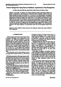
5 Experimental Results We design three sets of recognition experiments, all using input data from the CUReT database, which is a collection of BTF/BRDF measurements for 61 real-world textured surfaces, each imaged under more than 200 different combinations of viewing and illumination directions. The first experiment is devised to analyze the dependency of the image texton method performance on two factors: the cardinality of the image texton library, and the dimensionality of the universal eigenspace
��
obtained by performing PCA on the set of image texton histograms corresponding to the set of training
��#
texture images. To construct the image texton library, we consider �
Figure 14 (a). For each sample we employ a set of
�
�
3D texture samples, shown in
unregistered texture images corresponding to
distinct imaging conditions, given in Table 5 and illustrated in Figures 22 and 23. These images are uni-
� , illustrated in Figure
formly sampled from the complete set of 205 texture images available within the CUReT database for each texture sample. Every texture image is filtered by filter bank
�
of size
� � �
�
#
12. To ensure that only texture information is included for analysis, all texture images are manually preseg-
20
Recognition Rate
0.99 0.98 0.97 0.96 0.95 0.94 0.93 0.92 250 200 150 100 50 Number of Eigen Vectors
0
100
200
300
400
500
600
Number of K-Means
Figure 13: Recognition rate, i.e. the percentage of correctly classified test images, as a function of the cardinality of the image texton library, as well as of the number of dimensions of the eigenspace. mented and converted to grey level. Color is not used as a cue for recognition because we are specifically studying the performance of texture models. Moreover, we consider that the use of color greatly assists the recognition since many of the surface samples in the CUReT dataset are well separated in color space. For
�� . In
computational reasons, the filter responses corresponding to a pixel in the image are grouped for each of the three scales to form three feature vectors. Three feature spaces are defined, each of dimension
�
�
�
� ��� �� � � � � �� # # �� �� � � �� � , therefore we
each of the feature spaces, k-means algorithm is used to determine the cluster centers. We varied the number of cluster centers
�
over the set of values
�
created ten image texton libraries for each scale.
���#
We consider for recognition the same image texton libraries. The subset of
�� ��
�
�
�
�
��
�
�
�
�
�
�
�
�
3D texture samples as the ones used for creating the
texture images, for each sample, used for constructing the
image texton library, are also employed during training. The set of texton histograms, corresponding to �
�
�
�
texture images used for training, is employed to compute the universal eigenspace via
PCA. In all our experiments, PCA is accomplished by employing the SLAM software library (Nene et al., 1994) (Murase and Nayar, 1995). We construct texture models by projecting all texton histograms onto the universal eigenspace, and by fitting a curve to the projected points corresponding to a certain sample using a quadratic b-spline interpolation. Therefore, each 3D texture sample is represented in the parametric
21
eigenspace by a manifold indexed by the imaging parameters. We experiment with multiple values for the dimensionality of the eigenspace, specifically we vary from 30 to 250, with a step of 10. For classification we use 19 arbitrarily chosen texture images for each 3D textured surface, so the total number of test images is 380. Note that the sets of imaging conditions corresponding to the test and training images are disjoint. The recognition rate, expressed as the percentage of correctly classified texture images, is analyzed in terms of its dependency on two factors: the size of the image texton library, and the number of eigenvectors. The plotted surface, illustrated in Figure 13, clearly suggests that undersampling the image texton library negatively affects the performance of the method. This behavior is due to grouping distinct local structural characteristics to be represented by the same image texton, affecting the capability of the representation to discriminate between different 3D textured surfaces. The number of eigenvectors also influences the performance, i.e. when the dimensionality of the eigenspace is reduced under a certain level the representation does not preserve the discriminative properties of the image texton histograms, and the performance decreases. However, when the size of the image texton library is above 300 and the set of image texton histograms is projected onto an eigenspace of dimensionality greater than 70, the performance is excellent. Specifically, for this experiment, the recognition rate is well above 98%. The second experiment is more complex and it is designed to analyze the dependency of the image texton method on the number of texture images used for training. This experiment also analyzes the efficiency of representing the BTF through the compacted version, obtained as we propose in Section 2.3. The image
. Again, the recognition experiment utilizes the
texton library employed during the second experiment is one of the versions computed during the first experiment, i.e. the image texton library of size
�
�
same set of 3D texture samples as for creating the image texton library, illustrated in Figure 14. For each
� ), for which the texture image is almost featureless, �� � images for each therefore their recognition becomes very difficult. The resulting subset consists of �
sample we now consider the entire BTF, with the exception of the texture images corresponding to very tilted poses (polar angle of viewing direction
��
��
�
�
texture sample, therefore the entire set of texture images processed during the second experiment is of size 3120. To design the training stage of the image texton recognition method, we compute the compact represen-
�� �
tation of the BTF for each 3D texture sample. The compacted BTF is obtained by processing the entire BTF to compute the reference manifold
� �� �
�
, based on all
22
�
�
�
points in the parametric eigenspace
1
Recognition Rate
0.9 0.8 0.7 0.6 0.5 0.4 10
20 30 40 50 Number of training images for each sample
(a)
(b)
Figure 14: (a) The set of 20 3D texture samples used for creating the image texton library. First row: sample 1 (felt), sample 4 (rough plastic), sample 6 (sandpaper), sample 10 (plaster-a), sample 12 (rough paper); second row: sample 14 (roofing shingle), sample 16 (cork), sample 18 (rug-a), sample 20 (styrofoam), sample 22 (lambswool); third row: sample 25 (quarry tile), sample 27 (insulation), sample 30 (plaster-b zoomed), sample 33 (slate-a), sample 35 (painted spheres); fourth row: sample 41 (brick-b), sample 45 (concrete-a), sample 48 (brown bread), sample 50 (concrete-c), sample 59 (cracker-b). The image texton library should be generic enough to represent a large class of 3D texture samples, while it should also be comprehensive enough to allow good segregation between different classes of texture. (b) Recognition rates for individual 3D texture samples (solid lines), and the global recognition rate (thick dashed line), as a function of the number of training images for each sample. of texton histograms. As described in Section 2.3, we determine for each 3D texture sample the subset of significant texture images which best encode the local structural features of the surface. The constraint imposed for obtaining the compact representation of the BTF is consistent across the entire set of surfaces,
�� ��
� ��
� ��
�
, retained as and it is defined in Equations 1, 2, 3. The distance between the reduced-by- manifold � �� � �� the compacted BTF, and the reference manifold , does not exceed of the maximum distance
�����
�
between any of the reduced-by- manifolds
��
�
� ��
,
�
� � �
� � � , and � �� �
�
.
In the first column of Figure 16, for six different 3D textured surfaces: sample 4 (rough plastic), sample 10 (plaster-a), sample 20 (styrofoam), sample 22 (lambswool), sample 45 (concrete-a), and sample 50 (concrete-c), we illustrate the profile of the distance
�
defined as
����� �
�
��� ��� � � � � �� 23
between
� � �
�
��
��� ��
and
� �� �
�
, normalized by
��� � (4)
��
���
��
���
felt
0.285
-2.377
1.371
-0.041
rough plastic
0.810
-2.702
0.615
-0.685
sandpaper
1.209
-2.984
0.393
-1.571
plaster-a
0.196
3.141
0.982
0.000
rough paper
1.101
-2.433
1.358
-0.281
roofing shingle
0.196
3.141
1.374
0.000
cork
0.196
3.141
1.374
0.000
rug-a
0.196
3.141
1.374
0.000
styrofoam
0.213
-1.410
0.473
-0.431
lambswool
0.196
3.141
0.982
0.000
quarry tile
0.393
3.141
0.785
0.000
insulation
0.196
3.141
1.374
0.000
plaster-b zoomed
1.101
-2.433
1.358
-0.281
slate-a
1.178
3.141
1.178
0.000
painted spheres
0.196
3.141
0.982
0.000
brick-b
0.393
3.141
0.785
0.000
concrete-a
0.196
3.141
0.982
0.000
brown bread
0.196
3.141
1.374
0.000
concrete-c
0.196
3.141
0.982
0.000
cracker-b
0.196
3.141
1.374
0.000
Sample
�� �� ����� �
�� � �
Table 1: Viewing and illumination directions ( , in radians) for the most significant texture images corresponding to each of the samples involved during the second experiment. as a function of the ordinal index of the eliminated point on the manifold. It is interesting to observe that the removal of various points from the manifold affects differently the profile of the plot
�
vs. . Also,
consider samples 45 and 50, respectively concrete-a and concrete-c. It is noticeable that the profiles of the plots
�
vs. corresponding to these two samples are qualitatively similar, while the two surfaces, illustrated
in Figure 16, have similar intrinsic nature, presenting analogous local structural features. These observations show that the differences in the local structure of various surfaces are reflected by the differences between corresponding eigenspace representations. That is, 3D texture samples which have different local structures have compact representations of BTF defined by distinct imaging parameters.
24
Felt
Rough plastic
Sandpaper
Plaster-a
Rough paper
Roofing shingle
Cork
Rug-a
Styrofoam
Lambswool
Quarry tile
Insulation
Plaster-b zoomed
Slate-a
Painted spheres
Brick-b
Concrete-a
Brown bread
Concrete-c
Cracker-b
Figure 15: Illustration of the viewing direction (marked by ’*’, in blue) and the illumination direction (marked by ’+’, in red) for the most significant texture images corresponding to each sample involved in recognition during the second experiment. The corresponding imaging conditions are characterized by the �� �� ����� �
� � � angles (in radians) listed in Table 1.
�
��
� ��
In the second column of Figure 16, for the same six 3D texture samples, we show the profiles of distance �
between
�
�
and
� ��
, normalized by
� ��
defined in Equation 3, as a function of the number
�
of eliminated points from the manifold. Note that for some samples the threshold , defined in Equation �
2, is reached sooner, while other samples show a slower growth of the profile samples have different cardinalities for the compacted BTF. Let
��
sample 10,
for sample 20,
�
#
�
for sample 22,
�
���
�� �
denote the number of significant texture
��
images within the compacted BTF of a 3D texture sample. We have that �
vs. . As a result different
�
for sample 4,
for sample 45, and
�
��
�
for
for sample
50. As we expect, the number of significant texture images required within the compact representation of
25
di
1 0.9 0.8 0.7 0.6 0.5 0.4 0.3 0.2 0.1 0
di
1 0.9 0.8 0.7 0.6 0.5 0.4 0.3 0.2 0.1 0
di
1 0.9 0.8 0.7 0.6 0.5 0.4 0.3 0.2 0.1 0
di
1 0.9 0.8 0.7 0.6 0.5 0.4 0.3 0.2 0.1 0
di
1 0.9 0.8 0.7 0.6 0.5 0.4 0.3 0.2 0.1 0
di
1 0.9 0.8 0.7 0.6 0.5 0.4 0.3 0.2 0.1 0
1
1
1
1
20
20
20
20
40
40
40
40
60
60
60
60
80
i
80
i
80
i
80
di
1 0.9 0.8 0.7 0.6 0.5 0.4 0.3 0.2 0.1 0
di
1 0.9 0.8 0.7 0.6 0.5 0.4 0.3 0.2 0.1 0
di
1 0.9 0.8 0.7 0.6 0.5 0.4 0.3 0.2 0.1 0
di
1 0.9 0.8 0.7 0.6 0.5 0.4 0.3 0.2 0.1 0
di
1 0.9 0.8 0.7 0.6 0.5 0.4 0.3 0.2 0.1 0
di
1 0.9 0.8 0.7 0.6 0.5 0.4 0.3 0.2 0.1 0
100 120 140
100 120 140
100 120 140
20
40
60
80
100 120 140
20
40
60
80
1
1
20
20
20
20
40
40
40
40
60
60
60
60
80
i
80
i
80
i
80
100 120 140
Sample 10 (plaster-a)
100 120 140
Sample 20 (styrofoam)
100 120 140
Sample 22 (lambswool)
100 120 140
i
100 120 140
i
1
1
1
i
1
Sample 4 (rough plastic)
100 120 140
1
1
20
20
40
40
60
60
80
i
80
i
i
Sample 45 (concrete-a)
100 120 140
Sample 50 (concrete-c)
100 120 140
� ��
Figure 16: Samples 4 (rough plastic), 10 (plaster-a), 20 (styrofoam), 22 (lambswool), 45 (concrete-a), and � � � 50 (concrete-c). First column: the distance between the reference manifold and the reduced ��� � � � manifolds , normalized by , vs. the ordinal index of the eliminated point. Second column: � �� � �� the distance between the reference manifold and the reduced manifolds ,normalized by , vs. the number of eliminated points. Third column: each 3D textured surface illustrated by the corresponding most significant texture image determined by reducing the manifold. Notice how well the local structure of the surface is captured by the most important texture image within the BTF.
��
�����
�����
� ��
26
��
1
2
3
4
5
6
7
8
9
10
11
12
9
14
18
21
25
28
32
36
42
45
51
56
180
280
360
420
500
560
640
720
840
900
1020
1120
2940
2840
2760
2700
2620
2560
2480
2400
2280
2220
2100
2000
��� ����� � � � �� ����
�
Table 2: The number of significant texture images considered for each of the 3D texture samples (first row), and the corresponding cardinality � of the training set for each sample (second row). The total number of ����� ��� ��������� training and testing images are listed on third and fourth rows, respectively.
�
the BTF correlates well with the visual complexity of the surface. In practice, we store the manifolds as a list of multidimensional points acquired by sampling at high rate the parametric curve in the eigenspace obtained by fitting a quadratic b-spline interpolation to a set of knot points. The distance between two manifolds is determined by computing the average over the set
� ��
of point-to-point distances between two corresponding points on the manifolds, given that both manifolds
� based on �
are sampled at the same rate. However, consider the reference manifold
��
�
�
and some reduced manifold
�
� ��
, based on
�
knot points,
knot points, sampled at the same rate. We employ
SLAM to perform PCA, interpolation, and manifold sampling. During sampling, SLAM keeps constant the number of sampled points between two neighboring knot points. Consequently, the distance between �
two manifolds is dependent on the relative position of the missing points on
�� �
�
, i.e. removal of knot
points closer to the end points of the manifold generates a larger distance between the two manifolds, while removal of knot points close to the middle point affects less the configuration of the manifold. Therefore
� �� �
this comparison between
�
�
and
��
� ��
is invalid, because it does not capture any information about the
texture structure. Our solution for this problem is to replace an eliminated knot point with a point obtained
� � �
by linearly interpolating its two neighbors. That is, we locally flatten the manifold. Consequently, the manifolds
� �� �
�
,
��
���
�
�
or
of knot points of the manifold
�� �
�
,
�
� �� ��
� ��
� � �
are all based on
�
consists of
�
knot points. As an example, the set
points lying on the line between the two end points
of the manifold, in the multidimensional eigenspace. From the second column of Figure 16 it is detectable that the profile of the plot �
The nonmonotonicity of
�
vs. is not monotonic.
is always observed for large values of , i.e. after a large number of points have
been already eliminated from the manifold. The reduced manifolds, based on less than about 15% of the original number of knot points, become very unstable, i.e. they lose important topological information about 27
0.7
0.35
d153
0.3
D153(k) D154(k)
0.6
d 154 0.25
0.5
0.2
0.4
d i 0.15
Di (k)0.3
0.1
0.2
0.05
0.1
0
0
20
40
60
80
0
100 120 140 160
x 10
0
2
4
6
8
10
i
16 18
2
20
k
(a)
� ��
12 14
(b) �
� ��
� ��
�
�� �� �� � ���#
� ��
vs. , for sample 1 (felt). The circled region shows that� the distance Figure 17: (a)� The plot of distance � � � � ��� � � ��� ��� � between and is larger than the distance between and . (b) The � plots � � � � � � ��� � of point-to-point distances between each of the reduced-bymanifolds , where , � � �� the point on the manifold. Note that for most and the reference � ��� , as � a � function of the index � of � � � � ��� � � ��� � , i.e. the points on are further away from , than the points values of� ���, ��� � ��� on .
� ��
�
� ��
� ��
�
�
the original manifolds. As a result, �
consider the plot of
vs.
��
�� �
�
is closer to
� ��
� ��
�� �
�
than
�
, when
� �� �
�
. As an example,
����
for sample 1 (felt), depicted in Figure 17(a). Note that
���� , that is
�
�� � ���# , between ��
the reduced manifold based on the last three points is further away from the reference than the reduced
�� � ���# , and the reference manifold � ��
manifold based only on the endpoints. The point-to-point distances ���
�
�
� ��
�
� �
�
�
�
,
, as a function of the index
Figure 17(b). It can be observed that for many values of � , we have that
�
����
�
�
�
�
�
�
,
of the point, are plotted in � �
�
� �
�
���� �
�
�
. Again, this
behavior is present when the reduced-by- manifolds rely on too few initial knot points and do not preserve anymore the global structural configuration captured by the reference manifold. The third column of Figure 16 illustrates the most significant texture image corresponding to each sample. We expect the significant image to be the image which best conveys the physical structure of the surface. Indeed, visual observations support this conjecture. For each 3D texture sample, the most significant image shown in the third column of Figure 16 clearly depicts detailed local surface structure. This observation suggests that the compact representation of the BTF indeed consists of the subset of texture images which best convey the surface texture. The construction of a compact representation of the BTF is important for an efficient design of the training
28
Figure 18: Sample 4 (rough plastic) imaged under various viewing and illumination conditions. The appearance changes so dramatically with the camera/illumination directions, that the images seem to be from different surfaces. These texture images show that, because of surface structure, a large number of texture images are necessary to represent the compacted BTF for this 3D texture sample. set employed for recognition. We study the performance variation of the image texton recognition method as a function of the number of important texture images used for training. We construct 12 variants of training sets, by varying the size of the compact representation of the BTF for each sample. The number
�
�� . To determine the global training set we take the union over all 20 surface samples
of significant texture images considered for each 3D texture sample is increased from 1 to 12, with a step of 1, i.e.
�
�
� � � �
of all individual sets of
�
most significant imaging conditions for each sample. Explicitly, consider that
�
�
each texture image is captured under particular imaging conditions, uniquely determined by the quadruple � ���� � � ��� �
� � � � � of imaging parameters . If a texture image, characterized by a certain , belongs to any � of the compacted BTFs, then the global training set will contain the texture image characterized by for
�
all 3D texture samples. For reference, this procedure used for determining the global training set is referred to as the merging procedure. By varying
�
from 1 to 12 we obtain various values for the size of the global
training set, denoted by � , as listed on second row of Table 2. Therefore we have 12 variants for the second
� �
�� � �
recognition experiment, where each experiment uses a subset of � texture images for training, and a subset of
�
�
�
�� �
� texture images for testing. The testing set is the complement of the training set relative � �
to the entire available BTF, consisting of
�
texture images. The sizes of the overall training sets � ��� �� � � ��� ��� and the corresponding overall testing sets, i.e. and , respectively, are specified on the third and
�
fourth rows of Table 2. Note that, while in this work we employ information about the imaging conditions in order to design the training sets, generally the image texton recognition method does not require knowledge about the viewing/illumination parameters. Usually the training sets are arbitrarily chosen from the sampled BTF, as in (Cula and Dana, 2001b) (Cula and Dana, 2002) (Cula et al., 2003). The reason for using the imaging conditions during training is to test the efficiency of representing the textured surface based on the compacted BTF.
29
Figure 14 (b) depicts the profiles of the global and individual recognition rates, as percentages of correctly
��
recognized images, indexed by the number of training images considered for each sample. As we enrich the training set with more texture images, the recognition rate increases. By employing
� �
� �
�
most significant
���
images within each BTF, and by applying the merging procedure we obtain a global training set consisting � � ��� ��� � � � of � texture images for each sample. The total set employed for training consists of � ��� ��� � images, while during testing a total set of novel texture images are classified. This particular
��
�
configuration of the system achieves an excellent global recognition rate of over 96%. It is notable that four 3D texture samples (roofing shingle, rug-a, lambswool, cracker-b) were 100% correctly classified, while other eight samples (felt, sandpaper, rough paper, cork, insulation, painted spheres, brown bread, concretec) reached a recognition rate well above 97%. Moreover, all samples, with one exception, were correctly classified in a proportion larger than 90%. The exception corresponds to sample 4 (rough plastic), for which we achieved a recognition rate of 85%. This type of surface has a rich local structure, which leads to extreme variations of appearance as the imaging parameters are varied. Figure 18 presents a series of eight texture images of sample 4, obtained by sampling the BTF employed in our experiments. The performance obtained for sample 4 suggests that the image texton library involved in computing the 3D texture representation does not comprise key structural features which best convey the surface texture. It is also consistent that sample 4, among the complete set of 20 samples involved in the second experiment, necessitates the largest number of texture images for the compacted BTF, i.e. 76 texture images. This observation shows that our proposed texture representation performs well when encoding the structural complexity of the surface. In order to verify the validity of our method for determining the compacted BTF, we design an alternative recognition experiment. In this case we do not construct the training set by using the most significant texture images of each 3D texture sample, instead the training set is randomly sampled from the available BTF. We � , for which the training compare the performance of the alternative recognition experiment, denoted by set consists of 56 randomly chosen texture images for each sample, with the performance of the recognition experiment, denoted by
� � , for which the training set of the same size is designed by applying the merging
procedure to the set of the reduced BTF’s consisting of 12 most important texture images for each sample. � While achieves a global recognition rate of 96%, the alternate experiment shows a significantly
��
poorer performance of about 86% recognition rate. When the cardinality of the training set is decreased, as expected, the performance is also gradually
30
1
Recognition Rate
0.9 0.8 0.7 0.6 0.5 0.4
10
(a)
20 30 40 50 Number of training images for each sample
(b)
Figure 19: (a) The set of 20 3D texture samples employed during the third recognition experiment. First row: sample 2 (polyester), sample 3 (terrycloth), sample 5 (leather), sample 7 (velvet), sample 8 (pebbles); second row: sample 9 (frosted glass), sample 15 (aluminum foil), sample 17 (rough tile), sample 19 (rug-b), sample 21 (sponge); third row: sample 24 (rabbit fur), sample 36 (limestone), sample 37 (brick-a), sample 39 (human skin), sample 43 (salt crystals); fourth row: sample 44 (linen), sample 47 (stones), sample 52 (white bread), sample 54 (wood-a), sample 58 (tree bark). (b) Recognition rates for individual 3D texture samples (solid lines), and the global recognition rate (thick dashed line), as a function of the number of training images for each sample. diminished. However, let us consider the case when
�
�
�
�
, i.e. the global training set is constructed by
�� corresponding to the most significant texture
applying the merging procedure to the compacted BTF containing only the most significant texture image.
���
Table 1 enumerates the four imaging parameters images within the BTF for all
�
�
�� � � � � ��� � �
� , and consequently, ��� �� novel images.
samples. These imaging conditions are illustrated on the hemisphere �
���
of viewing/illumination directions in Figure 15. The global training set is of size � � ��� ��� � � � ������� � the total number of train images is . Testing is performed for
�
Given this very restricted representation, the global recognition rate is still close to 70%. This result shows the efficiency of our approach for planning the training set by considering the compact representation for each BTF. Finally, a third experiment is designed to verify the property of generality of the image texton library. To examine if the image texton library is generic enough to represent local structural characteristics of an extensive range of real-world 3D textured surfaces, we design a recognition experiment which employs for recognition a set of 3D texture samples distinct from the set of samples utilized for computing the 31
di
1 0.9 0.8 0.7 0.6 0.5 0.4 0.3 0.2 0.1 0
di
1 0.9 0.8 0.7 0.6 0.5 0.4 0.3 0.2 0.1 0
di
1 0.9 0.8 0.7 0.6 0.5 0.4 0.3 0.2 0.1 0
di
1 0.9 0.8 0.7 0.6 0.5 0.4 0.3 0.2 0.1 0
di
1 0.9 0.8 0.7 0.6 0.5 0.4 0.3 0.2 0.1 0
di
1 0.9 0.8 0.7 0.6 0.5 0.4 0.3 0.2 0.1 0
1
1
1
1
1
1
20
40
60
80
di
1 0.9 0.8 0.7 0.6 0.5 0.4 0.3 0.2 0.1 0
di
1 0.9 0.8 0.7 0.6 0.5 0.4 0.3 0.2 0.1 0
100 120 140
Sample 24 (rabbit fur)
1
20
40
60
20
20
20
20
20
40
40
40
40
40
60
60
60
60
60
80
i
80
i
80
i
80
i
80
100 120 140
1
20
40
60
1 0.9 0.8 0.7 0.6 i d 0.5 0.4 0.3 0.2 0.1 0 1
100 120 140
di
1 0.9 0.8 0.7 0.6 0.5 0.4 0.3 0.2 0.1 0
di
1 0.9 0.8 0.7 0.6 0.5 0.4 0.3 0.2 0.1 0
di
1 0.9 0.8 0.7 0.6 0.5 0.4 0.3 0.2 0.1 0
100 120 140
100 120 140
100 120 140
80
100 120 140
i
i
1
1
1
20
20
20
20
40
40
40
40
60
60
60
60
80
i
80
i
80
i
80
i
80
Sample 39 (human skin)
100 120 140
Sample 43 (salt crystals)
100 120 140
Sample 44 (linen)
100 120 140
Sample 52 (white bread)
100 120 140
Sample 54 (wood-a)
100 120 140
i
i
�� � ��
��
Figure 20: Samples 24 (rabbit fur), 39 (human skin), 43� (salt crystals), 44 (linen), 52 (white bread), and � � � � � � � 54 (wood-a). First column: the distance between and , normalized by , vs. . Second � � � �� column: the distance between and , normalized by , vs . Third column: each texture surface is illustrated by the corresponding most significant texture image determined by reducing the manifold. Again, the local structure is well exhibited by the most significant images.
� ��
32
�����
� ��
�
� � �
� �
polyester
1.209
-2.984
0.393
-1.571
terrycloth
0.196
3.141
0.982
0.000
leather
0.285
-2.377
1.371
-0.041
velvet
0.437
-2.701
0.196
-1.571
pebbles
0.196
3.141
0.982
0.000
frosted glass
0.393
3.141
0.785
0.000
aluminum foil
0.196
3.141
0.982
0.000
rough tile
0.810
-2.702
0.615
-0.685
rug-b
0.196
3.141
0.982
0.000
sponge
0.196
3.141
0.982
0.000
rabbit fur
0.196
3.141
0.982
0.000
limestone
0.196
3.141
0.982
0.000
brick-a
0.196
3.141
0.982
0.000
human skin
0.196
3.141
0.982
0.000
salt crystals
0.196
3.141
0.982
0.000
linen
0.628
-1.795
0.662
-1.136
stones
0.196
3.141
0.982
0.000
white bread
0.196
3.141
0.982
0.000
wood-a
0.717
-1.271
0.877
-0.767
tree bark
0.196
3.141
0.982
0.000
Sample
�� �� ����� �
�� � �
Table 3: Viewing and illumination directions ( , in radians) for the most significant texture images corresponding to each of the samples involved in recognition during the third experiment.
� � ������ � � � �� ����
1
2
3
4
5
6
7
8
9
10
11
8
11
17
22
27
34
39
44
48
51
56
160
220
340
440
540
680
780
880
960
1020
1120
2960
2900
2780
2680
2580
2440
2340
2240
2160
2100
2000
�
Table 4: The number of significant texture images considered for each of the 3D texture samples (first row), and the corresponding cardinality � � of��� the training set for each sample (second row), for the third � ������� ��� experiment. The total number of training and testing images are listed on third and fourth rows, respectively.
�
33
Polyester
Terrycloth
Leather
Velvet
Pebbles
Frosted glass
Aluminum foil
Rough tile
Rug-b
Sponge
Rabbit fur
Limestone
Brick-a
Human skin
Salt crystals
Linen
Stones
White bread
Wood-a
Tree bark
Figure 21: Illustration of the viewing direction (marked by ’*’, in blue) and the illumination direction (marked by ’+’, in red) for the most significant texture images corresponding to each sample involved in recognition during the third experiment. The corresponding imaging conditions are characterized by the �� �� ����� �
� � � angles (in radians) listed in Table 3.
��
texton library. The collection of 3D texture samples involved for classification is illustrated in Figure 19 (a), and consists of
�
�
samples: sample 2 (polyester), sample 3 (terrycloth), sample 5 (leather),
sample 7 (velvet), sample 8 (pebbles), sample 9 (frosted glass), sample 15 (aluminum foil), sample 17 (rough tile), sample 19 (rug-b), sample 21 (sponge), sample 24 (rabbit fur), sample 36 (limestone), sample 37 (brick-a), sample 39 (human skin), sample 43 (salt crystals), sample 44 (linen), sample 47 (stones), sample 52 (white bread), sample 54 (wood-a), sample 58 (tree bark). The setup of the third recognition
�� �
experiment is similar to the one of the second experiment. We employ the same texton library, and we proceed similarly by using
�
���
texture images within each BTF. Each BTF is analyzed to compute
34
the corresponding compacted representation. Table 3 and Figure 21 enumerate the imaging conditions corresponding to the most significant texture image for all 20 samples involved in recognition. The first
��
� ��
column of Figure 20 illustrates for samples 24 (rabbit fur), 39 (human skin), 43 (salt crystals), 44 (linen), �
52 (white bread), and 54 (wood-a), the plots of distance
����� , as a function of the ordinal index
� �
between
�
and
� ��
, normalized by
of the eliminated point on the manifold. Again, the profiles of
these plots show that the imaging conditions corresponding to the most important texture images within the BTF vary from one sample to another. Also, by visually examining the texture images illustrated in Figure 20 it is noticeable that the surfaces have distinct local structural features. This observation shows that the compact representation of the BTF correlates well with the surface local geometric characteristics, that is samples exhibiting distinct structural attributes have corresponding significant texture images captured under �
different imaging conditions. The distance
�
between
��
� ��
and
� �� �
�
, normalized by
��� � , indexed by
the number of eliminated points is depicted for all six samples of interest in the second column of Figure 20. These plots suggest that each surface, depending on its structural complexity, requires a specific number of significant texture images within its compacted BTF. For these six samples, the third column of Figure 20 shows the corresponding most important texture images within each BTF. Again, it is notable how well the local structural characteristics of surface are illustrated in these images. For this third experiment we construct 11 variants of global training sets, obtained by considering � � � � �
� �
most significant texture images within each BTF and by applying the merging procedure. The global
training sets have cardinalities as listed in Table 4. We investigate the performance of the system as the total � ��� ��� � ��� ��� number of training images and the total number of test images are varied as enumerated in the
�
�
third and fourth rows of Table 4. The recognition rate as a function of the size of the global training set
���
for each 3D texture sample is depicted in Figure 19 (b). When only the most significant texture image for � ��� ��� � � each sample is considered, we train the system on a total number of texture images, while � ��� ��� � novel texture images are used for classification. Though this representation is extremely
�
�� ��
simple, the global recognition rate is well above 70%. As the set of important images for each sample is expanded, the recognition rate increases, reaching 96% when the global training set contains 56 images for each surface. This global training set is obtained by applying the merging procedure when considering the most important 11 texture images per sample. These excellent classification results confirm the validity of the assumption that different 3D textured surfaces have similar local structural properties. Therefore
35
an image texton library obtained from a limited collection of 3D texture samples also conveys the texture characteristics of other surfaces. There are limitations of the texton library. For instance in our experiments we identify surfaces like sample 28 (crumpled paper) or sample 38 (ribbed paper), which exhibit structural characteristics not well represented by the texton library. As a result the texture models of these two samples are not well discriminated. This observation shows that the breadth of the image texton library is a considerable factor in designing efficiently the texture model we propose in this work.
6 Conclusion Due to the inherent microgeometry of the real world surfaces, the surface appearance varies significantly when the viewing and lighting directions change, due to effects such as shadowing, shading or local occlusions. Consequently, an efficient surface representation must account for these changes. In this work we introduce a BTF-based representation for 3D textured surfaces, termed bidirectional feature histogram (BFH). The construction of the BFH consists of two main tasks: first, the image texton library is created from a heterogeneous collection of surface samples such that basic image features, termed image textons, are well represented; second, a set of texture images is processed to obtain the surface model, that is a collection of image feature histograms, as a function of the imaging conditions. Based on the BFH, we have designed a quantitative evaluation for the level of relative significance of texture images within the BTF, allowing each BTF to be reduced to a core subset of texture images which best conveys the surface characteristics. We have developed a 3D texture recognition method which constructs a BFH-based surface model, and it classifies the surface based on a single novel texture image of unknown imaging parameters. Our recognition experiments, which utilized over 6200 texture images corresponding to 40 real-world surface samples from the CUReT database, show excellent classification results. The results are especially interesting when one considers that there is no need for a priori information about the imaging parameters during surface classification. The methods presented here have important implications for computer vision. For 3D texture recognition or classification, invariance to illumination or viewing direction is essential for robust performance. Our approach has the key advantages that a single image can be used for recognition without the need for iterative
36
methods and the viewing/illumination direction of the novel images need not be known. Furthermore, the images in the training set need not be registered. An additional impact of our work is the identification of a smaller subset of images from the CUReT database that can be used to sufficiently represent the texture class. The CUReT database contains over 200 images per sample and it is useful to determine which images can be considered redundant using a quantitative measure. Indeed this analysis can be used for BRDF/BTF measurement planning in subsequent experiments. The work described also has implications for computer graphics. Histograms of textural features have become an important building block for texture synthesis techniques. Compact representations of surface texture such as the one described here can be modified to support efficient and realistic rendering of natural objects with complex surface texture.
Acknowledgement This material is based upon work supported by the National Science Foundation under Grant No. 0092491 and Grant No. 0085864. We thank Thomas Leung for providing the filter bank used in his experiments.
37
��
���
��
���
No.
��
���
��
���
1
1.389
-1.970
1.374
-1.571
33
0.196
0.000
1.374
0.000
2
0.982
0.000
1.374
0.000
34
1.308
-1.978
1.370
-0.764
3
1.308
-1.163
1.371
-0.765
35
0.909
-1.517
1.357
-0.281
4
1.051
-0.417
1.358
-0.153
36
0.000
0.000
1.178
0.000
5
0.785
0.000
1.178
0.000
37
0.196
3.141
0.981
0.000
6
1.272
-2.496
1.154
-2.096
38
1.141
-2.514
0.955
-1.136
7
1.099
-1.476
1.154
-1.045
39
0.392
3.141
0.785
0.000
8
1.421
-3.015
1.130
-2.738
40
0.589
3.141
0.589
0.000
9
1.374
3.141
0.981
3.141
41
0.785
3.141
0.392
0.000
10
0.589
0.000
0.981
0.000
42
0.987
-3.007
0.284
-0.764
11
1.101
-2.432
0.955
-2.005
43
0.981
3.141
0.196
0.000
12
1.178
3.141
0.785
3.141
44
1.178
3.141
0.000
0.000
13
1.038
-3.013
0.662
-2.860
45
0.196
3.141
1.374
0.000
14
0.694
-2.211
0.589
-1.570
46
1.154
-2.096
1.360
-0.430
15
0.213
-1.410
0.472
-0.430
47
0.392
3.141
1.178
0.000
16
0.000
3.141
0.392
0.000
48
0.589
3.141
0.981
0.000
17
0.274
-2.335
0.284
-0.764
49
0.662
-2.860
0.955
-0.153
18
0.196
3.141
0.196
0.000
50
0.785
3.141
0.785
0.000
19
0.392
3.141
0.000
0.000
51
0.981
3.141
0.589
0.000
20
1.432
-2.365
1.374
-1.570
52
1.178
3.141
0.392
0.000
21
0.589
0.000
1.374
0.000
53
1.374
3.141
0.196
0.000
22
1.285
-1.570
1.370
-0.764
54
0.589
3.141
1.374
0.000
23
1.122
-1.226
1.360
-0.430
55
0.625
-2.857
1.370
-0.041
24
0.392
0.000
1.178
0.000
56
0.733
-2.628
1.360
-0.094
25
1.122
-1.914
1.154
-1.045
57
0.785
3.141
1.178
0.000
26
0.717
-1.267
1.130
-0.403
58
0.981
3.141
0.981
0.000
27
1.047
-2.526
0.785
-1.570
59
1.178
3.141
0.785
0.000
28
0.261
-2.202
0.662
-0.281
60
1.374
3.141
0.589
0.000
29
0.196
3.141
0.589
0.000
61
0.981
3.141
1.374
0.000
30
0.392
3.141
0.392
0.000
62
1.178
3.141
1.178
0.000
31
0.589
3.141
0.196
0.000
63
1.374
3.141
0.981
0.000
32
0.785
3.141
0.000
0.000
64
1.374
3.141
1.374
0.000
No.
� � � � � � � � �
Table 5: Viewing and illumination directions ( images used for creating the image texton library.
38
, in radians) corresponding to the set of texture
1
2
3
4
5
6
7
8
9
10
11
12
13
14
15
16
17
18
19
20
21
22
23
24
25
26
27
28
29
30
31
32
Figure 22: Illustration of the viewing (marked with blue ’*’) and illumination (marked with red ’+’) directions 1 - 32, as listed in Table 5. 39
33
34
35
36
37
38
39
40
41
42
43
44
45
46
47
48
49
50
51
52
53
54
55
56
57
58
59
60
61
62
63
64
Figure 23: Illustration of the viewing (marked with blue ’*’) and illumination (marked with red ’+’) directions 33 - 64, as listed in Table 5. 40
References Aksoy, S. and Haralick, R. M., 1999, “Graph-theoretic clustering for image grouping and retrieval”, Proceedings of the IEEE Conference on Computer Vision and Pattern Recognition 1, 63–68 Bovik, A. C., Clark, M., and Geisler, W. S., 1990, “Multichannel texture analysis using localized spatial filters”, IEEE Transactions on Pattern Analysis and Machine Intelligence 12 Chantler, M., 1995, “Why illuminant direction is fundamental to texture analysis”, IEE Proceedings Vision, Image and Signal Processing 142(4), 199–206 Cula, O. G. and Dana, K. J., 2001a, “Compact representation of bidirectional texture functions”, Proceedings of the IEEE Conference on Computer Vision and Pattern Recognition I, 1041–1047 Cula, O. G. and Dana, K. J., 2001b, “Recognition methods for 3D textured surfaces”, Proceedings of SPIE Conference on Human Vision and Electronic Imaging VI 4299, 209–220 Cula, O. G. and Dana, K. J., 2002, “Image-based skin analysis”, Proceedings of Texture 2002 - The 2nd international workshop on texture analysis and synthesis 35–40 Cula, O. G., Dana, K. J., Murphy, F. P., and Rao, B. K., 2003, “Skin texture modeling”, to appear in International Journal of Computer Vision Dana, K. J. and Nayar, S. K., 1998, “Histogram model for 3D textures”, Proceedings of the IEEE Conference on Computer Vision and Pattern Recognition 618–624 Dana, K. J. and Nayar, S. K., 1999a, “3D textured surface modeling”, IEEE Workshop on the Integration of Appearance and Geometric Methods in Object Recognition 46–56 Dana, K. J. and Nayar, S. K., 1999b, “Correlation model for 3D texture”, International Conference on Computer Vision 1061–1067 Dana, K. J., van Ginneken, B., Nayar, S. K., and Koenderink, J. J., 1997, “Reflectance and texture of real world surfaces”, Proceedings of the IEEE Conference on Computer Vision and Pattern Recognition 151–157 Dana, K. J., van Ginneken, B., Nayar, S. K., and Koenderink, J. J., 1999, “Reflectance and texture of real world surfaces”, ACM Transactions on Graphics 18(1), 1–34 Jain, A., Prabhakar, S., and Hong, L., 1999, “A multichannel approach to fingerprint classification”, IEEE Transactions on Pattern Analysis and Machine Intelligence 21(4), 348–369
41
Julesz, B., 1981, “Textons, the elements of texture perception and their interactions”, Nature (290), 91–97 Koenderink, J. J., van Doorn, A. J., Dana, K. J., and Nayar, S. K., 1999, “Bidirectional reflection distribution function of thoroughly pitted surfaces”, International Journal of Computer Vision 31(2-3), pp. 129–144 Leung, T. and Malik, J., 1999, “Recognizing surfaces using three-dimensional textons”, International Conference on Computer Vision 2, 1010–1017 Leung, T. and Malik, J., 2001, “Representing and recognizing the visual appearance of materials using three-dimensional textons”, International Journal of Computer Vision 43(1), 29–44 Liu, X., Yu, Y., and Shum, H., 2001, “Synthesizing bidirectional texture functions for real-world surfaces”, Proceedings of SIGGRAPH 97–106 Ma, W. Y. and Manjunath, B. S., 1996, “Texture features and learning similarity”, Proceedings of the IEEE Conference on Computer Vision and Pattern Recognition 425–430 McGunnigle, G. and Chantler, M. J., 2000, “Rough surface classification using first order statistics from photometric stereo”, Pattern Recognition Letters 21, 593–604 Murase, H. and Nayar, S. K., 1995, “Visual learning and recognition of 3-D objects from appearance”, International Journal of Computer Vision 5–24 Nene, S. A., Nayar, S. K., and Murase, H., 1994, “SLAM: A Software Library for Appearance Matching”, Technical Report CUCS-019-94 Proceedings of ARPA Image Understanding Workshop Penirschke, A., Chantler, M., and Petrou, M., 2002, “Illuminant rotation invariant classification of 3D surface textures using Lissajous’s ellipses”, Proceedings of Texture 2002 - The 2nd international workshop on texture analysis and synthesis , pp. 103–108 Puzicha, J., Hoffman, T., and Buchmann, J., 1999, “Histogram clustering for unsupervized image segmentation”, International Conference on Computer Vision 2, 602–608 Randen, T. and Husoy, J. H., 1999, “Filtering for texture classification: a comparative study”, IEEE Transactions on Pattern Analysis and Machine Intelligence 21(4), 291–310 Suen, P. and Healey, G., 1998, “Analyzing the bidirectional texture function”, Proceedings of the IEEE Conference on Computer Vision and Pattern Recognition 753–758 Suen, P. and Healey, G., 2000, “The analysis and recognition of real-world textures in three dimensions”, IEEE Transactions on Pattern Analysis and Machine Intelligence 22(5), 491–503 Tong, X., Zhang, J., Liu, L., Wang, X., Guo, B., and Shum, H.-Y., 2002, “Synthesis of bidirectional texture
42
functions on arbitrary surfaces”, Proceedings of SIGGRAPH 665–672 van Ginneken, B., Koenderink, J. J., and Dana, K. J., 1999, “Texture histograms as a function of irradiation and viewing direction”, International Journal of Computer Vision 31(2-3), 169–184 van Ginneken, B., Stavridi, M., and Koenderink, J. J., 1998, “Diffuse and specular reflectance from rough surfaces”, Applied Optics 37, 130–139 Varma, M. and Zisserman, A., 2002, “Classifying images of materials”, Proceedings of the European Conference on Computer Vision 255–271
43