Department of Computer Science, Cornell University, Ithaca, NY 14853 ... images from online photo collections, such as F
Location Recognition using Prioritized Feature Matching Yunpeng Li
Noah Snavely
Daniel P. Huttenlocher
Department of Computer Science, Cornell University, Ithaca, NY 14853 {yuli,snavely,dph}@cs.cornell.edu
Abstract. We present a fast, simple location recognition and image localization method that leverages feature correspondence and geometry estimated from large Internet photo collections. Such recovered structure contains a significant amount of useful information about images and image features that is not available when considering images in isolation. For instance, we can predict which views will be the most common, which feature points in a scene are most reliable, and which features in the scene tend to co-occur in the same image. Based on this information, we devise an adaptive, prioritized algorithm for matching a representative set of SIFT features covering a large scene to a query image for efficient localization. Our approach is based on considering features in the scene database, and matching them to query image features, as opposed to more conventional methods that match image features to visual words or database features. We find this approach results in improved performance, due to the richer knowledge of characteristics of the database features compared to query image features. We present experiments on two large city-scale photo collections, showing that our algorithm compares favorably to image retrieval-style approaches to location recognition. Key words: Location recognition, image registration, image matching, structure from motion
1
Introduction
In the past few years, the massive collections of imagery on the Internet have inspired a wave of work on location recognition—the problem of determining where a photo was taken by comparing it to a database of images of previously seen locations. Part of the recent excitement in this area is due to the vast number of images now at our disposal: imagine building a world-scale location recognition engine from all of the geotagged images from online photo collections, such as Flickr and street view databases from Google and Microsoft. Much of this recent work has posed the problem as that of image retrieval [1–4]: given a query image to be recognized, find a set of similar images from a database using image descriptors or visual features (possibly with a geometric verification step), often building on bag-of-words techniques [5–9]. In many such approaches, the database images are largely treated as independent collections of features, 1
This work was supported in part by NSF grant IIS-0713185, Intel, Microsoft, Google, and MIT Lincoln Laboratory.
2
Yunpeng Li, Noah Snavely, and Daniel P. Huttenlocher
and any structure between the images is ignored. In this paper we consider exploiting this potentially rich structure for use in location recognition. For instance, recent work has shown that it is possible to automatically estimate correspondence information and reconstruct 3D geometry from large, unordered collections of Internet images of landmarks and cities [10, 3, 11]. Starting with such structure, rather than a collection of raw images, as a representation for location recognition and localization is promising for several reasons. First, the point cloud is a compact “summary” of the scene—it typically contains orders of magnitude fewer points than there are features in an image set, in part because each 3D point represents a cluster of related features, but also because many features extracted by algorithms like SIFT are noisy and not useful for matching. Second, for each reconstructed scene point we know the set of views in which a corresponding image feature was detected, and the size of this set is related to the “stability” of that point, i.e., how reliably it can be detected in an image, as well as how visible that scene feature is (e.g., a point on a tower might be more visible than other features, see Figure 1). We can also determine how correlated two points are—i.e., how often they are detected in the same images. Finally, when using Internet photo collections to build our database, the number of times a given scene point is viewed is also related to the “popularity” of nearby viewpoints—some parts of a scene may be photographed much more often than others [12]. In this paper, we explore how these aspects of reconstructed photo collections can be used to improve location recognition. In particular, we use scene features (corresponding to reconstructed 3D points), rather than images, as matching primitives, revisiting nearest-neighbor feature matching for this task. While there is a history of matching individual features for recognition and localization [13–15], we advocate reversing the usual process of matching. Typically, image features are matched to a database of features. Instead, we match database features to image features, motivated by the richer information available about scene features relative to query image features. Towards this end, we propose a new, prioritized feature matching algorithm that matches a subset of scene features to features in the query image, ordered by our estimate of how likely a scene feature is to be matched given our prior knowledge about the feature database, as well as which scene features have been successfully matched so far. This prioritized approach allows “common” views to be localized quickly, sometimes with just a few hundred nearest neighbor queries, even for large 3D models. In our experiments this approach also successfully localizes a higher proportion of images than approaches based on image retrieval. In addition, we show that compressing the model by keeping only a subset of representative points is beneficial in terms of both speed and accuracy. We demonstrate results on large Internet databases of city images. Given the feature correspondences found using our algorithm, we estimate the exact pose of the camera. While this final step relies on an explicit 3D reconstruction, many of the ideas we present—e.g., finding stable features and prioritizing scene features for matching—only require knowledge of feature correspondences across the image database, and not 3D geometry per se. However, because we ultimately produce a camera pose, and because the global geometry imposes additional consistency constraints on the correspondences, we represent our scene with explicit geometry, and refer to our scene features as “points” and the collection of scene features as a “point cloud.”
Location Recognition using Prioritized Feature Matching
2
3
Related Work
Our work is most closely related to that of Irschara et al. [4], which also uses SfM point clouds as the basis of a location recognition system. Our work differs from theirs in several key ways, however. First, while they use a point cloud to summarize a location, their recognition algorithm is still based on an initial image retrieval step using vocabulary trees. In their case, they generate a minimal set of “synthetic” images that covers the point cloud, and, given a new query image, use a vocabulary tree to retrieve similar images in this covering. In one sense, our approach is the dual of [4]: instead of selecting a set of images that cover the 3D points, we select a minimal set of 3D points that cover the images, and use these points themselves as the matching primitives. Second, while [4] uses images taken by a single person, we use city-scale image databases taken from the Internet. Such Internet databases differ from more structured datasets in that have much wider variation in appearance, and also reflect the inherent “popularity” of given views. Our approach is sensitive to and exploits both of these properties. Our work is also related to the city-scale location recognition work of Schindler et al. [1], who use stability of visual words, as well as their distinctiveness, as cues for building a recognition database. As with [4], Schindler et al.use image retrieval as a basis for location recognition, and use a database of images taken a regular samples throughout a city. Like [4], [1], and [15], part of our approach involves reducing the amount of data used to represent locations, a theme which has been explored by other researchers as well. For instance, Ni et al.[16] use epitomes [17] as compact representations of locations created from videos of different scenes. Li et al. [3] use clustering to derive “iconic” images from large Internet photo collections, then localize query images by retrieving similar iconic images using bag-of-words or GIST descriptors [18]. Similarly, [19] builds a landmark recognition engine by selecting iconic images using a graph-based algorithm. Finally, a number of researchers have applied more traditional recognition and machine learning techniques the problem of location recognition [2, 20, 21]. Others have made use of information from image sequences; while this is a common approach in the SLAM (Simultaneous Localization and Mapping) community, human travel priors have also been used to georegister personal photo collections [22].
3
Building a Compact Model
Given a large collection of images of a specific area of interest (e.g., “Rome”) downloaded from the Internet, we first reconstruct one or more 3D models using image matching and structure from motion (SfM) techniques. Our reconstruction system is based on the work of Agarwal et al. [23]; we use a vocabulary tree to propose an initial set of matching image pairs, do detailed SIFT feature matching to find feature correspondences between images, then use SfM to reconstruct 3D geometry. Because Internet photos taken in cities tend to have high density near landmarks or other popular places, and low density elsewhere, a set of city photos often breaks up into several connected components (and a large number of “singleton” images that are not matched
4
Yunpeng Li, Noah Snavely, and Daniel P. Huttenlocher
Fig. 1. SIFT Features in an image corresponding to reconstructed 3D points in the full model (left) and the compressed model (right) for Dubrovnik. The feature corresponding to the most visible point (i.e., seen by the most number of images) is marked in red in the right-hand image. This feature, the face of a clock tower, is intuitively a highly visible one, and was successfully matched in 370 images (over 5% of the total database).
to any other photo—we remove these from consideration, as well as other very small connected components). For instance, the Rome dataset described in Section 5 consists of 69 large components. An example 3D reconstruction is shown in Figure 2. Each reconstruction consists of a set of recovered camera locations, as well as a set of reconstructed 3D points, denoted P . For each point p ∈ P , we know the set of images in which p was successfully detected and matched during the feature matching process (and deemed to be a geometrically consistent detection during SfM). We also have a 128-byte SIFT descriptor for each detection (we will assign the mean descriptor to p). Given a new query image from the same scene, our goal is to find correspondences between these scene features and the query image, then determine the camera pose. One property of Internet photo collections (and current SfM methods) is that there is a large variability in the number of times each scene feature is matched between images. While many scene points are matched in only two images, others might be successfully matched in hundreds. Consequently, not all scene features are equally useful when matching with a new query image. This suggests a first step of “compressing” the set of scene features by keeping only a subset of informative points, thus reducing the computational cost of matching and suppressing potential sources of confusion. A na¨ıve way to compress the model is to rank the scene features by “visibility” (by which we mean the number of images in which that point has been successfully detected and matched) and select a set from the top of this list. However, points selected in such way can (and usually do) have very uneven spatial distribution, with popular areas having a large number of points, and other areas having few or none. Instead, we would like to choose a set of points that are both prominent and that cover the whole model. To this end, we pose the selection of points as a set covering problem, where the images in the model are the elements to be covered and each point is regarded as a set containing the images in which it is visible. In other words, we seek the smallest subset of P , such that each image is covered by at least one point in the subset. Given such a subset, we might expect that a query image drawn from the same distribution of views as the database images would—roughly speaking—match
Location Recognition using Prioritized Feature Matching
5
Fig. 2. Reconstructed 3D point cloud for Dubrovnik, viewed from overhead. Left: full model. Right: compressed model (P c ). The bright red regions represent the distribution of reconstructed camera positions.
at least one point in the model. However, because feature matching is a noisy process, and because robust pose estimation requires more than one a single match, we instead require that the subset covers each image at least K times (e.g., where K = 100).1 Although computing the minimum set K-cover is NP-hard, a good approximation can be found using a greedy algorithm that always selects the point which covers the largest number of not-yet-fully covered images. Note that this is different from the covering problem in [4], which aims to cover the points instead of the images. Our covering criterion is also related to the informative features used in Schindler et al. [1], though our method is different; we choose features based on explicit correspondences from feature matching and SfM, and do not use a direct measure of feature distinctiveness. For our problem, given our initial point set P , we compute two different K-covers: one for K = 5 but limited to 2,000 points (via early stopping of the greedy algorithm), denoted P s , and one for K = 100 (without an explicit limit on the number of points), denoted P c . Intuitively, P s forms an extremely compact “seed” description of the entire model that can be quickly swept through to find promising areas in which to focus the search for further feature matches, while P c is a more exhaustive representation that can be used for more accurate localization. We describe how our matching algorithm uses these sets in the next section. In our experiments, the reduction of points from model compression is significant. For the Dubrovnik set, the point set was reduced from over 2 million in the full model to under 80,000 in the compressed model P c . Figure 1 shows the features corresponding to reconstructed 3D points in the full and the compressed Dubrovnik models that are visible in one particular image. The point clouds corresponding to the full and compressed models are shown in Figure 2.
4
Registration and Localization
The ultimate goal of our system is to produce an accurate pose estimate of a query image, given a relevant image database. To register a query image to the 3D model using pose estimation, we need to first find a set of correspondences between scene features 1
If an image sees fewer than K points in the full model, all of those points are selected.
6
Yunpeng Li, Noah Snavely, and Daniel P. Huttenlocher
in the (compressed) model and image features in the query image. While many recent approaches initially pose this as an image retrieval problem, we reconsider an approach based purely on directly finding correspondences using nearest-neighbor feature matching. In our case, we represent each point in our model with the mean of the corresponding image feature descriptors. While the mean may not necessarily be representative of clusters of SIFT features that are large or multi-modal, it is a commonly used approach for creating compact representations (e.g. in k-means clustering) and we have found this simple approach to work well in practice (though better cluster representations is an interesting area for future work). Given a set of SIFT descriptors in a query image (in what follows we refer to these as “features,” for simplicity) and a set of SIFT descriptors representing the points in our model (we will refer to these descriptors as “points”), we consider two basic matching strategies: – Feature-to-point matching, or F2P, where one takes each feature (in the query image), and finds the best matching point (in the database) and – Point-to-feature matching, or P2F, where one conversely matches points in the model to features in the query image. At first glance, F2P matching seems like the natural choice, since we usually think of matching a query to a database—not vice versa—and even the compressed model is usually much larger than the set of features in a single image. However, P2F matching has the desirable property that we have a significant amount of information about how informative each database point is, and which database points are likely to appear together, while we do not necessarily have much prior information about the features in an image (other than low-level confidence measures provided by the feature detector). In fact, counter to intuition, we show that P2F matching can be made to find matches more quickly than F2P—especially for popular images—by choosing an intelligent priority ordering of the points in the database, such that we often only need to consider a relatively small subset of the model points before sufficient matches are found. We evaluate the empirical performance of F2P and P2F matching in Section 5. For both matching strategies, we find potential matches using the approximate nearest neighbor search [24]. As in prior work, we found that the priority search algorithm worked well in pratice. We used a fixed search limit of 250 points per query; increasing the search limit did not lead to significantly better results in our experiments. We use a modified version of the ratio test that is common in nearest neighbor matching to classify a match as true or false. For P2F matching, we use the usual ratio test: a match between a point p from the model and feature f from the query image is dist(p,f ) considered a true match if dist(p,f 0 ) < λ, where dist(·, ·) is the distance between the 0 corresponding SIFT descriptors, f is the second nearest neighbor of p among features in the query image, and λ is the threshold ratio (0.7 in our implementation). For F2P matching, we found that the analogous ratio test does not perform as well. We speculate that this might be because the number of points in the compressed model is larger (and hence denser) than the typical image feature set, and this increased density in SIFT space has an effect on the ratio test. Instead, given a feature f and its approximate nearest neighbor p in the model, we compute the second nearest neighbor f 0 to p in the
Location Recognition using Prioritized Feature Matching
7
dist(f,p) image, and threshold on the ratio dist(f 0 ,p) (note that this ratio could be ≥ 1). We found this test to perform better for F2P matching. For P2F matching, we could find correspondences by applying the above procedure to every point in the compressed model. However, this would be very costly. We can do much better by prioritizing certain queries over others, as we describe next.
4.1
Prioritized Point-to-feature (P2F) Matching
As noted earlier, each point in the reconstructed 3D model is associated with the set of images in which it is successfully detected and matched (“visible”). Topologically, the model can be regarded as a bipartite graph (which we call the visibility graph) where each point and each image is a vertex, and where the edges encode the visibility relation. Based on this relation, we develop a matching algorithm guided by three heuristics: 1. Points with higher degree in the visibility graph should generally be considered before points with lower degree, since a highly visible point is intuitively more likely to be visible in a query image. Our matching algorithm thus maintains a priority for each point, initially equal to its degree in the visibility graph. 2. If two points are often visible in the same set of images, and one of them has been matched to some feature in the query image, then the other should be more likely to find a match as well. 3. The algorithm should be able to quickly “explore” the model before “exploiting” the first two heuristics, so as to avoid being trapped in some part that is irrelevant to the query image. To this end, a set of highly visible seed points (corresponding to P s in Section 3) are selected as a preprocess; these seed points are the basis for an initial exploratory round of matching (before moving on to the more exhaustive P c model). We limit the size of P s to 2,000 points, which is somewhat arbitrary but represents a balance between exploration and exploitation. Our P2F matching algorithm matches model points to query features in priority order (using a priority queue), always choosing the point with the highest priority as the next candidate for matching. The priorities of all points P are initially set to be proportional to their degrees in the visibility graph, i.e. di = j Vij . The priorities of the “seed” points are further increased by a sufficiently large constant, so that all seed points rank above the rest. Whenever the algorithm finds a match to a point p that passes the ratio test, it increases the priority of related points, i.e., points seen in the same images as p. Thus, if the algorithm finds a true match, it can quickly home in on the correct part of the model and find additional true matches. If a true match is found early on (especially likely with a popular image), the image can be localized with a relatively small number of comparisons. The matching algorithm terminates (successfully) once it has found a sufficient number of matches (given by a parameter N ), or (unsuccessfully) when it has tried to match more than 500N points. On success, the matches are passed onto the pose estimation routine. The abort criterion is based on our empirically observed “background” match rate of roughly 1/500, i.e., in expectation every one out 500 points will succeed the ratio test and be matched to some feature purely by chance (see also Section 5). Hence when 500N points have been tried, the rate of finding matches so far is
8
Yunpeng Li, Noah Snavely, and Daniel P. Huttenlocher
Algorithm 1: Prioritized P2F Matching Input: set of seed points P s and compressed points P c , n-by-m visibility matrix V , a query image Output: Set of matches M Parameters: Number of uniquely matched features required N , weight factor ω M, Y ← ∅ (* Initialize the set of matches M and uniquely matched features Y *) P For all i (i = 1 · · · n), Si ← di , where di = j Vij (* Initialize priorities S *) For all i ∈ P , Si is incremented by a sufficiently large constant t←0 while max S > 0 and |Y | < N do i ← arg max S, t ← t + 1 Search for an admissible match among the features in the query image for Xi if such a feature y is found do M ← M ∪ {(Xi , y)}, and Y ← Y ∪ {y} for each j, s.t. Vij = 1 do (* Update the priorities *) for each k, s.t. Vkj = 1 do Sk ← Sk + ω/di end for end for end if Si ← −∞ If t ≥ 500N , abort end while
no higher than the background rate and hence a strong indication that the number of outlier matches will be very large and hence the image will most likely not be recognized by the model. The algorithm also depends on a second parameter ω, which is the trade-off between the static (first) heuristic and dynamic (second) heuristic. A higher value of ω makes the priority of a point depend more on how well nearby points (in the visibility graph) have been matched, and less on its inherent visibility (i.e. its degree); a zero value for ω, on the other hand, would disable dynamic priorities altogether. We set ω = 10, which heavily favors the dynamic priorities. Our full algorithm for prioritized point-to-feature matching is given in Algorithm 1. We use a value N = 100, which appears to be sufficient for subsequent localization. In the case that the output M contains duplicates, i.e., multiple points are matched to the same feature, only the closest match (in terms of the distance between their SIFT descriptors) is kept. Although the update of priorities that corresponds to the two nested inner loops of Algorithm 1 may seem to be a significant extra computational cost, these updates only occur when a match is found. The overhead is further reduced by updating the priorities only at fixed intervals, i.e., after every certain number of iterations (100 in our implementation). This also allows the algorithm to be conveniently parallelized or ported to a GPU, though we have not yet implemented these enhancements.
Location Recognition using Prioritized Feature Matching
4.2
9
Feature-to-point (F2P) Matching
For feature-to-point (F2P) matching, it is not clear if any ordering of image features is better than another. Therefore all features in the query image are considered for matching. In our experiments, we find that not considering all features always decreases the registration performance of F2P matching in our experiments. 4.3
Camera Pose Estimation
If the matching algorithm terminates successfully, then the set of matches M links 2D features in the query image directly to 3D points in the model. These matches are fed into our pose estimation routine. We use the 6-point DLT approach to solve for the projection matrix of the query camera, followed by a local bundle adjustment to refine the pose.
5
Experiments
We evaluated the performance of our method on three different image collections. Two of the models, Dubrovnik and Rome, were built from Internet photos retrieved from Flickr; the third, Vienna, was built from photos taken by a single calibrated camera (the same dataset used in [4]). Figure 2 shows part of the reconstructed 3D model for Dubrovnik. For each dataset, the number of registered images was in the thousands, and the number of 3D points in the full model in the millions; statistics are shown in Table 1. Table 1. Statistics for each 3D model. Each row lists the name of the model, the number of cameras used in its construction, the number of points, and number of connected components in the reconstruction. Model # Cameras Dubrovnik 6844 Rome 16,179 Vienna 1,324
# Points # CCs 2,208,645 1 4,312,820 69 1,132,745 3
In order to obtain relevant test images (i.e. images that can be registered) for Dubrovnik and Rome, we first built initial models using all available images. A random subset of the images that were accepted by the 3D reconstruction process was then removed from these initial models and withheld as test images. This was done by removing their contribution to the SIFT descriptors of any points they see, as well as deleting any points that are no longer visible in at least two images. The resulting model no longer has any information about the test images, while we can still use the initial camera poses as “ground truth.” For Dubrovnik and Rome, we also included the relevant test images of the other data set as negative examples. In all our experiments no irrelevant images were falsely registered. For Vienna, the set of test images are the same Internet photos
10
Yunpeng Li, Noah Snavely, and Daniel P. Huttenlocher
Table 2. Results for Dubrovnik. The test set consists of 800 relevant images and 1000 irrelevant ones (from Rome). Images NN queries by P2F Time in seconds registered registered rejected registered rejected Compressed model (76645 points)
Full model (1975263 points)
P2F F2P Combined
753 667 753
9756 -
46433 -
0.73 1.62 0.70
2.70 1.62 3.96
Seedless P2F Static P2F Basic P2F
747 693 699
9986 16722 16474
46332 46558 46661
0.75 1.11 1.09
2.69 2.68 2.69
P2F F2P Combined
735 595 742
7379 -
49588 -
1.08 2.75 1.12
3.84 2.75 5.83
Seedless P2F Static P2F Basic P2F
691 610 605
7620 21345 21117
49499 49628 49706
1.13 1.53 1.52
3.86 3.03 3.04
Vocab. tree (all features) Vocab. tree (points only)
677 652
-
-
1.4 1.3
4.0 4.0
as used in [4] (these images were not used in building the model). In all cases, the test images are downsampled to a maximum of 1600 pixels in both width and height. The Vienna data set is different from Dubrovnik and Rome in that it is taken by the same camera over a short period of time, and is much more controlled, uniformly sampled, and homogeneous in appearance. Thus, it does not necessarily generalize as well to diverse query images, such as the Internet photos used in the test set (e.g, the stability of a point in the model may not necessarily be a good predictor of its stability in an arbitrary query image). Indeed, we found that using a model compressed with K = 100 for this collection was not adequate, likely because a covering for each image in the model may not also cover a wide variety of images with different appearance. Hence we used a larger covering (K = 1000) for this data set. Other than this, all parameters of the our algorithm are the same throughout the experiments. As an extra validation step, we also created a second model for Vienna in the same way as we did for Dubrovnik and Rome, first building an initial model including all images, then removing the test images. We found that the model created in this way performed no better than the one built without ever involving the test images. This suggests that our evaluation methodology for Dubrovnik and Rome does not favorably bias the the results. For each dataset, we evaluated the performance of localization and pose estimation using a number of algorithms. These include our proposed method and several of its variants, as well as a vocabulary tree-based image retrieval approach [6]. For each experiment, we accept a pose estimate as successful if at least twelve inliers to a recovered pose are found (we also discuss localization accuracy below). As in [4], we did not find false positives at this inlier rate (though some cameras had high localization error due to poor conditioning). The results of our experiments are shown in Table 2 - 4. For
Location Recognition using Prioritized Feature Matching
11
Table 3. Results for Rome. The entire test set consists of 1000 relevant images and 800 irrelevant ones (from Dubronik). Images NN queries by P2F Time in seconds registered registered rejected registered rejected Compressed model (144777 points)
Full model (4067119 points)
P2F F2P Combined
921 796 924
12963 -
46756 -
0.91 1.72 0.87
2.93 1.72 4.67
Seedless P2F Static P2F Basic P2F
888 805 808
13841 21490 21300
46779 46966 47150
0.96 1.35 1.35
2.93 2.87 2.88
P2F F2P Combined
863 788 902
11253 -
49500 -
1.57 2.91 1.67
4.34 2.91 7.20
Seedless P2F Static P2F Basic P2F
769 682 681
10287 23548 23409
49635 49825 49887
1.52 1.77 1.78
4.33 3.34 3.34
Vocab. tree (all features) Vocab. tree (points only)
831 815
-
-
1.2 1.2
4.0 4.0
matching strategies, “F2P” and “P2F” denote feature-to-point and point-to-feature, respectively, as described in Section 4. In “Combined”, we use P2F first and, if pose estimation fails, rerun with F2P. The other three variants are simply stripped-down versions of P2F (Algorithm 1), with no seed points (“seedless”), with no dynamic prioritization (“static”), or with neither (“basic”). These are included to show how much performance is gained through each enhancement. For Dubrovnik and Rome, the results for the vocabulary tree approach are obtained using our own implementation, using a tree of depth five and branching factor ten (i.e., with 100,000 leaf nodes). For each query image, we retrieve the top 10 images from the vocabulary tree, then perform detailed SIFT matching between the query and candidate image (similar to [4], but using actual images). We tested two variants, one in which all image features are used, and one using only features which correspond to points in the 3D model. When sufficient matches are found, we estimate the pose of the query camera given these matches. All times for our implementation are based on running a single-threaded process on a 2.8GHz Xeon processor. For P2F matching, we show the average number of nearestneighbor queries as well as running time for both images that are registered and those that fail to register. For F2P, however, these numbers are essentially the same for both cases since we exhaustively match image features to the model. The results in the tables show that our point matching approach achieves significantly higher registration rates (without false positives) than the state of the art in 3D location recognition [4], as well as the vocabulary tree variants we tried. Among various matching strategies, the P2F approach (Algorithm 1) performs significantly better than its F2P counterpart. In some cases the results can be further improved by combining both together, at the expense of extra computation time. Although one might
12
Yunpeng Li, Noah Snavely, and Daniel P. Huttenlocher Table 4. Results for Vienna. Images NN queries by P2F Time in seconds registered registered rejected registered rejected
Compressed model (200638 points)
Full model (1132745 points)
P2F F2P Combined
204 145 205
6245 -
32920 -
0.55 2.04 0.54
1.96 2.04 3.62
Seedless P2F Static P2F Basic P2F
182 164 166
6201 14393 14274
34360 39664 40056
0.54 0.97 0.94
2.07 2.30 2.33
P2F F2P Combined
190 136 196
4289 -
41530 -
0.63 2.78 0.71
2.85 2.78 5.32
Seedless P2F Static P2F Basic P2F Vocab. tree (from [4])
160 162 161 164
4034 16164 16134 -
44263 45388 45490 -
0.59 3.00 1.11 2.72 1.11 2.67 ≤ 0.27 (GPU)
think the P2F would be slower than F2P (since there are generally more 3D points in the model than features per image), this turns not to be the case. The experiments show that utilizing the extra information associated with the points makes P2F both faster and more accurate than F2P. The P2F variants that lack either dynamic priorities or seeding points, or both, perform much worse than the full algorithm, which illustrates the importance of these enhancements. Moreover, the compressed models generally perform at least as well as, if not better than, the full models, while being on average an order of a magnitude smaller in size. Hence they are able to save storage space and computation time without sacrificing accuracy. For the vocabulary tree approach, the two variants we tested are comparable, though using all image features gave somewhat better performance than using just the features corresponding to 3D points in our tests. One further property of the P2F method is that when it recognizes an image (i.e. is able to register it), it does so very quickly—much more quickly than in the case when the image is not recognized—since if a true match is found among the seed points, the algorithm generally only needs to consider a small subset of points. This resembles the ability of humans to quickly recognize a familiar place, while deciding that a place is unknown can take longer. Note that even in the case where the image is not recognized, our methods is still comparable in speed to the vocabulary tree based approach in terms of equivalent CPU time, although vocabulary tree methods can be made much faster by utilizing the GPU; [4] reports that a GPU implementation sped up their algorithm by a factor of 15-20. Our point matching approach is also amenable to GPU techniques. 5.1
Localization Accuracy
To evaluate localization accuracy we geo-registered the initial model for Dubrovnik so that each image receives a camera location in real-world coordinates, which we treat as noisy ground truth. The estimated camera location of each registered image is then
Location Recognition using Prioritized Feature Matching
13
compared with this ground truth, and the localization error is simply the distance between the two locations. For our results, this error had a mean of 18.3m, a median of 9.3m, and quartiles of 7.5m and 13.4m. While 87 percent of the images have errors below the mean, a small number were rather far off (up to around 400m in the worst case). This is most likely due to errors in estimated focal lengths (most likely for both the test image and the model itself), to which location estimates are very sensitive.
6
Summary and Discussions
We have demonstrated a prioritized feature matching algorithm for location recognition that leverages the significant amount of information that can be estimated about scene features using image matching and SfM techniques on large, heterogeneous photo collections. In contrast to prior work, we use points, rather than images, as a matching primitive, based on the idea that even a small number of point matches can convey very useful information about location. Our system is also able to utilize other cues as well. While we primarily consider the visibility of a point when evaluating its relevance, another important cue is its distinctiveness, i.e., how well it can predict a single location (a feature on a stop sign, for instance, would not be distinctive). While we did not observe problems due to repetitive features spread around a city model, one future direction would be to incorporate distinctiveness into our model (as in [15] and [1]). Our system is designed for Internet photo collections. While these collections are useful as predictors of the distribution of query photos, they typically do not cover entire cities. Hence many possible viewpoints may not be recognized. It will be interesting to augment such collections with more uniformly sampled photos, such as those on Google Street View or Microsoft Bing Maps. Finally, while we found that our system works well on city-scale models built from Internet photos, one question is how well it scales to the entire world. Are there features in the world that are stable and distinctive enough to predict a single location unambiguously? How many seed points do we need to ensure good coverage, at least of the popular areas around the globe? Answering such questions will reveal interesting information about the regularity (or lack thereof) of our world.
References 1. Schindler, G., Brown, M., Szeliski, R.: City-scale location recognition. In: Proc. IEEE Conf. on Computer Vision and Pattern Recognition. (2007) 2. Hays, J., Efros, A.A.: im2gps: estimating geographic information from a single image. In: Proc. IEEE Conf. on Computer Vision and Pattern Recognition. (2008) 3. Li, X., Wu, C., Zach, C., Lazebnik, S., Frahm, J.M.: Modeling and recognition of landmark image collections using iconic scene graphs. In: Proc. European Conf. on Computer Vision. (2008) 4. Irschara, A., Zach, C., Frahm, J.M., Bischof, H.: From structure-from-motion point clouds to fast location recognition. In: CVPR. (2009) 5. Sivic, J., Zisserman, A.: Video Google: A text retrieval approach to object matching in video s. In: Proc. Int. Conf. on Computer Vision. (2003) 1470–1477
14
Yunpeng Li, Noah Snavely, and Daniel P. Huttenlocher
6. Nist´er, D., Stew´enius, H.: Scalable recognition with a vocabulary tree. In: Proc. IEEE Conf. on Computer Vision and Pattern Recognition. (2006) 2118–2125 7. Chum, O., Philbin, J., Sivic, J., Isard, M., Zisserman, A.: Total recall: Automatic query expansion with a generative feature model for object retrieval. In: Proc. Int. Conf. on Computer Vision. (2007) 8. Philbin, J., Chum, O., Isard, M., Sivic, J., Zisserman, A.: Lost in quantization: Improving particular object retrieval in large scale image databases. In: Proc. IEEE Conf. on Computer Vision and Pattern Recognition. (2008) 9. Perdoch, M., Chum, O., Matas, J.: Efficient representation of local geometry for large scale object retrieval. In: Proc. IEEE Conf. on Computer Vision and Pattern Recognition. (2009) 10. Snavely, N., Seitz, S.M., Szeliski, R.: Photo tourism: Exploring image collections in 3d. In: SIGGRAPH. (2006) 11. Agarwal, S., Snavely, N., Simon, I., Seitz, S.M., Szeliski, R.: Building rome in a day. In: ICCV. (2009) 12. Simon, I., Snavely, N., Seitz, S.M.: Scene summarization for online image collections. In: Proc. Int. Conf. on Computer Vision. (2007) 13. Se, S., Lowe, D., Little, J.: Vision-based mobile robot localization and mapping using scaleinvariant features. In: Proc. Int. Conf. on Robotics and Automation. (2001) 2051–2058 14. Zhang, W., Kosecka, J.: Image based localization in urban environments. In: International Symposium on 3D Data Processing, Visualization and Transmission. (2006) 15. Li, F., Kosecka, J.: Probabilistic location recognition using reduced feature set. In: Proc. Int. Conf. on Robotics and Automation. (2006) 16. Ni, K., Kannan, A., Criminisi, A., Winn, J.: Epitomic location recognition. IEEE Trans. on Pattern Analysis and Machine Intelligence 31 (2009) 2158–2167 17. Jojic, N., Frey, B.J., Kannan, A.: Epitomic analysis of appearance and shape. In: Proc. Int. Conf. on Computer Vision. (2003) 34–41 18. Oliva, A., Torralba, A.: Modeling the shape of the scene: A holistic representation of the spatial envelope. Int. J. of Computer Vision 42 (2001) 145–175 19. Zheng, Y.T., Zhao, M., Song, Y., Adam, H., Buddemeier, U., Bissacco, A., Brucher, F., Chua, T.S., Neven, H.: Tour the world: building a web-scale landmark recognition engine. In: Proc. IEEE Conf. on Computer Vision and Pattern Recognition. (2009) 20. Crandall, D., Backstrom, L., Huttenlocher, D., Kleinberg, J.: Mapping the world’s photos. In: Proc. Int. World Wide Web Conf. (2009) 21. Li, Y., Crandall, D.J., Huttenlocher, D.P.: Landmark classification in large-scale image collections. In: Proc. Int. Conf. on Computer Vision. (2009) 22. Kalogerakis, E., Vesselova, O., Hays, J., Efros, A.A., Hertzmann, A.: Image sequence geolocation with human travel priors. In: Proc. Int. Conf. on Computer Vision. (2009) 23. Agarwal, S., Snavely, N., Simon, I., Seitz, S.M., Szeliski, R.: Building rome in a day. In: Proc. Int. Conf. on Computer Vision. (2009) 24. Arya, S., Mount, D.M.: Approximate nearest neighbor queries in fixed dimensions. In: ACM-SIAM Symposium on Discrete Algorithms. (1993)