4.2.3 Testing hypothesis about a single linear combination of the parameters. 17
... In order to test a hypothesis in statistics, we must perform the following steps:.
4 Hypothesis testing in the multiple regression model Ezequiel Uriel Universidad de Valencia Version: 09-2013 4.1 Hypothesis testing: an overview 4.1.1 Formulation of the null hypothesis and the alternative hypothesis 4.1.2 Test statistic 4.1.3 Decision rule 4.2 Testing hypotheses using the t test 4.2.1 Test of a single parameter 4.2.2 Confidence intervals 4.2.3 Testing hypothesis about a single linear combination of the parameters 4.2.4 Economic importance versus statistical significance 4.3 Testing multiple linear restrictions using the F test. 4.3.1 Exclusion restrictions 4.3.2 Model significance 4.3.3 Testing other linear restrictions 4.3.4 Relation between F and t statistics 4.4 Testing without normality 4.5 Prediction 4.5.1 Point prediction 4.5.2 Interval prediction 4.5.3 Predicting y in a ln(y) model 4.5.4 Forecast evaluation and dynamic prediction Exercises
1 2 2 3 5 5 16 17 21 21 22 26 27 28 29 30 30 30 34 34 36
4.1 Hypothesis testing: an overview Before testing hypotheses in the multiple regression model, we are going to offer a general overview on hypothesis testing. Hypothesis testing allows us to carry out inferences about population parameters using data from a sample. In order to test a hypothesis in statistics, we must perform the following steps: 1) Formulate a null hypothesis and an alternative hypothesis on population parameters. 2) Build a statistic to test the hypothesis made. 3) Define a decision rule to reject or not to reject the null hypothesis. Next, we will examine each one of these steps. 4.1.1 Formulation of the null hypothesis and the alternative hypothesis Before establishing how to formulate the null and alternative hypothesis, let us make the distinction between simple hypotheses and composite hypotheses. The hypotheses that are made through one or more equalities are called simple hypotheses. The hypotheses are called composite when they are formulated using the operators "inequality", "greater than" and "smaller than". It is very important to remark that hypothesis testing is always about population parameters. Hypothesis testing implies making a decision, on the basis of sample data, on whether to reject that certain restrictions are satisfied by the basic assumed model. The restrictions we are going to test are known as the null hypothesis, denoted by H0. Thus, null hypothesis is a statement on population parameters. 1
Although it is possible to make composite null hypotheses, in the context of the regression model the null hypothesis is always a simple hypothesis. That is to say, in order to formulate a null hypothesis, which shall be called H0, we will always use the operator “equality”. Each equality implies a restriction on the parameters of the model. Let us look at a few examples of null hypotheses concerning the regression model: a)
H0 : 1=0
b)
H0 : 1+ 2 =0
c)
H0 : 1=2 =0
d)
H0 : 2+3 =1
We will also define an alternative hypothesis, denoted by H1, which will be our conclusion if the experimental test indicates that H0 is false. Although the alternative hypotheses can be simple or composite, in the regression model we will always take a composite hypothesis as an alternative hypothesis. This hypothesis, which shall be called H1, is formulated using the operator “inequality” in most cases. Thus, for example, given the H0: H0 : j 1
(4-1)
H1 : j 1
(4-2)
we can formulate the following H1 :
which is a “two side alternative” hypothesis. The following hypotheses are called “one side alternative” hypotheses H1 : j 1
(4-3)
H1 : j 1
(4-4)
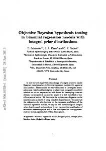
4.1.2 Test statistic A test statistic is a function of a random sample, and is therefore a random variable. When we compute the statistic for a given sample, we obtain an outcome of the test statistic. In order to perform a statistical test we should know the distribution of the test statistic under the null hypothesis. This distribution depends largely on the assumptions made in the model. If the specification of the model includes the assumption of normality, then the appropriate statistical distribution is the normal distribution or any of the distributions associated with it, such as the Chi-square, Student’s t, or Snedecor’s F. Table 4.1 shows some distributions, which are appropriate in different situations, under the assumption of normality of the disturbances. TABLE 4.1. Some distributions used in hypothesis testing.
Known
2
Unknown
2
1 restriction
1 or more restrictions
N
Chi-square
Student’s t
Snedecor’s F
2
The statistic used for the test is built taking into account the H0 and the sample data. In practice, as 2 is always unknown, we will use the distributions t and F. 4.1.3 Decision rule We are going to look at two approaches for hypothesis testing: the classical approach and an alternative one based on p-values. But before seeing how to apply the decision rule, we shall examine the types of mistakes that can be made in testing hypothesis. Types of errors in hypothesis testing In hypothesis testing, we can make two kinds of errors: Type I error and Type II error. Type I error We can reject H0 when it is in fact true. This is called Type I error. Generally, we define the significance level () of a test as the probability of making a Type I error. Symbolically,
Pr( Reject H 0 | H 0 )
(4-5)
In other words, the significance level is the probability of rejecting H0 given that H0 is true. Hypothesis testing rules are constructed making the probability of a Type I error fairly small. Common values for are 0.10, 0.05 and 0.01, although sometimes 0.001 is also used. After we have made the decision of whether or not to reject H0, we have either decided correctly or we have made an error. We shall never know with certainty whether an error was made. However, we can compute the probability of making either a Type I error or a Type II error. Type II error We can fail to reject H0 when it is actually false. This is called Type II error.
Pr( No reject H 0 | H1 )
(4-6)
In words, is the probability of not rejecting H0 given that H1 is true. It is not possible to minimize both types of error simultaneously. In practice, what we do is select a low significance level. Classical approach: Implementation of the decision rule The classical approach implies the following steps: a) Choosing . Classical hypothesis testing requires that we initially specify a significance level for the test. When we specify a value for , we are essentially quantifying our tolerance for a Type I error. If =0.05, then the researcher is willing to falsely reject H0 5% of the time. b) Obtaining c, the critical value, using statistical tables. The value c is determined by .
3
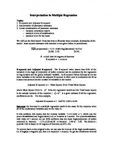
The critical value (c) for a hypothesis test is a threshold to which the value of the test statistic in a sample is compared to determine whether or not the null hypothesis is rejected. c) Comparing the outcome of the test statistic, s, with c, H0 is either rejected or not for a given . The rejection region (RR), delimited by the critical value(s), is a set of values of the test statistic for which the null hypothesis is rejected. (See figure 4.1). That is, the sample space for the test statistic is partitioned into two regions; one region (the rejection region) will lead us to reject the null hypothesis H0, while the other will lead us not to reject the null hypothesis. Therefore, if the observed value of the test statistic S is in the critical region, we conclude by rejecting H0; if it is not in the rejection region then we conclude by not rejecting H0 or failing to reject H0. Symbolically, If
sc
reject
If
sc
not reject H 0
H0
(4-7)
If the null hypothesis is rejected with the evidence of the sample, this is a strong conclusion. However, the acceptance of the null hypothesis is a weak conclusion because we do not know what the probability is of not rejecting the null hypothesis when it should be rejected. That is to say, we do not know the probability of making a type II error. Therefore, instead of using the expression of accepting the null hypothesis, it is more correct to say fail to reject the null hypothesis, or not reject, since what really happens is that we do not have enough empirical evidence to reject the null hypothesis. In the process of hypothesis testing, the most subjective part is the a priori determination of the significance level. What criteria can be used to determine it? In general, this is an arbitrary decision, though, as we have said, the 1%, 5% and 10% levels for are the most used in practice. Sometimes the testing is made conditional on several significance levels. Non Rejection Region NRR
Rejection Region RR
c
W
FIGURE 4.1. Hypothesis testing: classical approach.
An alternative approach: p-value With the use of computers, hypothesis testing can be contemplated from a more rational perspective. Computer programs typically offer, together with the test statistic, a probability. This probability, which is called p-value (i.e., probability value), is also known as the critical or exact level of significance or the exact probability of making a 4
Type I error. More technically, the p value is defined as the lowest significance level at which a null hypothesis can be rejected. Once the p-value has been determined, we know that the null hypothesis is rejected for any p-value, while the null hypothesis is not rejected when p-value, while the null hypothesis is not rejected when