BULLETIN of the
Bull. Malays. Math. Sci. Soc. (2) 27 (2004), 207−215
MALAYSIAN MATHEMATICAL SCIENCES SOCIETY
Significance Testing in Exact Logistic Multiple Regression MEZBAHUR RAHMAN AND SHUVRO CHAKROBARTTY Minnesota State University, Mankato, MN 56001, USA e-mail:
[email protected] and
[email protected]
Abstract. Exact logistic regression is discussed for multiple regressors. The exact significance of a regressor is computed which can be used in simplifying the model and/or to compute the significance of a variable or a set of variables in the model. Bilingual education data is analyzed using the procedure mentioned in this paper. 2000 Mathematics Subject Classification: 62J02
1. Introduction Following Cox ([1], Ch. 4), Tritchler [8] implemented an algorithm for the exact logistic regression analysis of a single regressor. Tritchler [8] used Fourier transformation algorithm given by [7] to compute the p value for testing the significance of the regression parameter. Mehta et al. [4] gave an efficient Monte Carlo method by networking the possible regressor values. We assume that we have a set of independent variables (regressors) that are to be used for prediction in each of the following situations: (1) predicting whether a company's dealer will soon be mired in dire financial straits, (2) predicting if a person is likely to develop heart disease, (3) predicting whether a hospital patient will survive until being discharged, or (4) predicting whether a person has achieved a desirable competency level of a learning. In such scenarios, the response (dependent) variable is binary. Due to a wide range of applications, the binary response models are studied explicitly. For the latest developments in the area, the reader is referred to [6], [2] and the references therein. Let X 1 , X 2 , , X p be p separate regressors and Y be a response (dependent) variable. Y can only take the values of ‘1’ for ‘success’ and ‘0’ for ‘failure’. A random sample of n data points is taken from a phenomenon. A general binary model is assumed as P ( Yi = 1) = π i = E ( Yi | X 1i , X 2i ,
, X pi ) , i = 1,2, … , n,
where 0 ≤ π i ≤ 1 and P (Yi = 0) = 1 − π i . We define the logistic model as
(1)
208
M. Rahman and S. Chakrobartty
π (x i ) = where β 0 , β 1 ,
(
exp β 0 + ∑ pj=1 β j x ji
(
)
1 + exp β 0 + ∑ pj=1 β j x ji
=
)
(
exp ∑ pj= 0 β j x ji
(
)
1 + exp ∑ pj= 0 β j x ji
)
(2)
, β p are unknown constants and x i is the row vector ( 1 x1i
x pi ) .
Notice that there is no error term on the right side of (2) because the left side is a function of E ( Y | X 1 , X 2 , , X p ), instead of Y, which serves to remove the error term. If y1 , y 2 ,
, y n is an observed binary sequence of size i, then
(
P Y1 = y1 , Y2 = y 2 ,
, Yn = y n | x11 , x12 ,
=
n
n
i =1
i =1
, x1n , x 21 , x 22
(
exp β 0 s + ∑ pj=1 β j t j
(
(
)
,x 2 n
∏ in=1 1 + exp β 0 + ∑ pj=1 β j x ji
where s = ∑ y i and t j = ∑ y i x ji
for j = 1, 2,
))
,x p1 ,x p 2 ,
,x pn
,
)
(3)
Following Cox (1970),
, p. n
n
i =1
i =1
inference is based on the sufficient statistics S = ∑ Yi and T j = ∑ Yi X ji for j = 1, 2,
, p , whose joint distribution is obtained by summing over all binary
sequences generating each realization of s, t1 , t 2
(
P S = s,T1 = t1 , T2 = t 2 ,
)
, Tp = t p =
, t p . Thus
(∏
) ( (1 + exp (β
p j =1
∏ in=1
), ))
C j exp β 0 s + ∑ pj=1 β j t j 0
+ ∑ pj =1 β j x ji
(4)
where C j ’s are the numbers of distinct binary sequences yielding the values s and t j ’s for the sufficient statistics. Exact inferences containing β j ’s may be based on the conditional
distribution
P ( T1 = t1 , T2 = t 2 ,
, T p = t p | S = s) .
Because
of
properties of the exponential family of distributions, the critical region defined by the upper tail values of t j within the conditional reference set provides a uniformly most powerful unbiased test of H 0 : β j = β j 0 versus H a : β j > β j 0 (Lehman 1959, p. 136). The conditional distribution used to test hypotheses concerning β j is
(
)
P Tj = t j | S = s =
C j exp ( β j 0 t j )
∑ C jl exp ( β j 0 t jl ) ∀l
where l is an index ranging over all the values taken by T j .
,
(5)
209
Significance Testing in Exact Logistic Multiple Regression
2. Tests of significance In one-sided tests, such as H 0 : β j = β j 0 versus H a : β j > β j 0 , the p value can be computed as
(
)
P Tj ≥ t j | S = s =
∑ Ci exp ( β j 0 t i )
i :T j ≥ t j
(6)
∑ Cl exp ( β j 0 t l ) ∀l
which tests for significance of the particular variate in the model. Due to the pattern of products of frequencies and exponentiation of a linear function, the p values are easy to compute for the significance of a set of variates. For example, for testing, H 0 : β j = β j 0 and β k = β k 0 versus H a : at least one of the β ’s not equal to the specified value can be tested by computing the p value as
(
( = 1 − P (T j ∉ R j ) P(Tk ∉ Rk ) = 1 − (1 − 2 P ( T j
P T j ∈ R j or Tk ∈ Rk | S = s
( 1 − 2 P ( Tk
)
= 1 − P T j ∉ R j and Tk ∉ Rk | S = s
≥ tk | S = s))
≥ t j |S = s
))
) (7)
where R j and Rk are the respective critical regions. The computations of such p values are demonstrated using a data set in Section 5. In equation (7) ' ≥ ' will be replaced in one or both places by ' ≤ ' depending on whether observed t j and/or t k lie in which tail of the distributions of T j and Tk . Similar processes can be applied for testing a set of more than two parameters.
3. Inferences based on maximum likelihood Maximum likelihood parameter estimation is studied extensively. Here we review the method as given in [5]. The log-likelihood function for the logit model (2) can be written as log L( β ) =
n
∑ { yi log π ( X i ) + (1 − yi )
i =1
log [1 − π ( X i )] },
where β is vector valued. For methods with more than one parameter, the first-order conditions require that we simultaneously solve the p + 1 equations uj =
δ log L( β ) = 0 , j = 0, 1, δβj
p
210
for which
M. Rahman and S. Chakrobartty
h jk =
δ 2 log L( β ) < 0, ( j = 0, 1, δβ j δβ k
, p), ( k = 0, 1,
, p) .
For the first-order conditions for the logit model (2), the likelihood expressions are written as
δ log L( β ) = U (β ) = δβ
n
∑ [ yi i =1
− π ( X i )] X i
and the negative of the second derivatives are I (β ) = −
δ 2 log L( β ) = δβδβ ′
n
∑ π (X i ) [1 − π (X i )] X′i X i
i =1
where U ( β ) is a ( p + 1) × 1 vector and I ( β ) is a ( p + 1) × ( p + 1) matrix. The matrix I ( β ) plays a key role in the estimation procedure and yields the estimated variances and covariances of the estimates as by-product. The asymptotic variances and covariances of the logit estimates are obtained by inverting the Hessian (or expected Hessian) matrix or information matrix I ( β ) . Then the Newton-Raphson iterative solution of a system of equations can be used to obtain the solutions of β ’s. At the tth iteration, estimates are obtained as
[(
βˆ (t ) = βˆ (t −1) + I βˆ (t −1)
)]
−1
(
)
U βˆ (t −1) .
The least square estimates of β ’s are often used as the initial estimates. The quantity βˆ k Dkk has asymptotic normal distribution where Dkk is the kth diagonal element of [ I ( βˆ )]−1 and can be used in testing and in forming confidence intervals for a particular parameter β k . Also, any subset of parameters can be tested using the following
asymptotic χ 2 statistic.
χ 2 = − [ log L1 − log L0 ] ,
(9)
has approximate χ 2 distribution with (n − q − 1) − (n − p − 1) = p − q degrees of freedom, where q + 1 is the number of unknown parameters in the model under the null hypothesis, log L1 is the maximized log likelihood under the full model, and log L0 is the maximized log likelihood under the null hypothesis.
211
Significance Testing in Exact Logistic Multiple Regression
4. Motivation Exact logistic regression is not a new phenomenon but in the wake of computational convenience is attracting more attention than before. Specialized software are not popular as they do not communicate effectively with the users. The algorithms are used in the software and are suggested by different authors are approximations, often through fourier transformations. Here we give algorithms to compute exact p values without any approximation. A data set is used to apply the exact logistic regression procedures. The exact p values will help to determine whether the particular factor is significant or not more accurately that using approximate t statistic for the maximum likelihood estimate. When particular factors are found to be significant then maximum likelihood method should be used in estimating or predicting the success probabilities. Often, the method of discriminant analysis (see [2], Section 1.5) gives higher rate of successful predictions but lacks properties like unbiasedness, consistency, and efficiency. Table 1. Estimated Variance-Covariance Matrix (MLE) ^
^
^
^
β0
β1
β2
β3
β0
0.8144
−0.0404
−0.1553
−0.0218
β1
^
−0.0404
0.0203
−0.0007
0.0025
^
−0.1553
−0.0007
0.0395
−0.0007
−0.0218
0.0025
−0.0007
0.0042
Statistics ^
β2 ^
β3
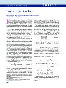
5. Application The population studied is thirteen schools of the Salinas City Elementary School district in the County of Monterey in California. Participating students were fifth and sixth graders of limited English proficiency. This study was undertaken in 1996 to take an in depth look at the data gathered for the population of limited English proficient students and its role in redesignating students to fluent English proficiency status. Information on 257 participating students were recorded and displayed in Table 3. In Tables 3, “E” represents English score, “S” represents Spanish score, “Y” represents the number of years in the program and “B” represents the redesignation in the bilingual status. In the variable “B”, ‘1’ indicates success of the participant in the program and ‘0’ indicates failure. In the variables “E” and “S”, higher the score means higher the proficiency. Redesignation in the program is done by the evaluator after considering the three variables “E”, “S” and “Y”, and the personal judgement of the evaluator. Here we will model using Logistic regression models. Goal is to give a rule by which one can be redesignated. The assumption is that the redesignation of the present data is done by an
212
M. Rahman and S. Chakrobartty
expert and future redesignation is possible by an auto-mated rule with the help of the present analysis. The Logistic model given in (2) is estimated using the maximum likelihood method (MLE) given in Powers ([5], Section 3.3.3) as described in Section 3 as
πˆ =
exp ( 1.0999 + 0.0127 Eng − 0.1816 Spa − 0.0474 Yrs) 1 + exp ( 1.0999 + 0.0127 Eng − 0.1816 Spa − 0.0474 Yrs)
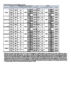
The variance-covariance matrix for the estimates of the parameters is computed using the delta method as [ I ( βˆ )] −1 in Section 3 and displayed in Table 1. The maximum likelihood estimates and the corresponding p values are displayed in Table 2. In Table 2, the likelihood ratio statistic as in (9) is represented as χ 2 , Est. represents the MLE estimates of the parameters, Z is the studentized statistic, p z is the p value for Z statistic, p χ 2 is the p value using the χ 2 statistic, Exact p is the p value using the exact method as described in Section 2. In testing H 0 : β1 = 0 and β 2 = 0
Table 2. Estimates and p values
pχ2
0.9290
0.0078
0.9296
2 P (T1 ≥ 210 S = 138) = 0.8204
−0.9137
0.3609
0.8410
0.3591
2 P (T2 ≥ 553 S = 138) = 0.3889
0.7314
0.4645
0.5410
0.4620
2 P (T3 ≥ 673 S = 138) = 0.4177
Z
pz
βˆ 0
1.0999
1.2188
0.2229
βˆ
0.0127
0.0891
βˆ 2
−0.1816
βˆ 3
−0.0474
1
p
χ2
Est.
versus H a : at least one of β 1 and β 2 non-zero.
Exact
p value = 1 − (1 − 2 P(T1 ≥ 210)
S = 138)) ( 1 − 2P( T2 ≤ 553 S = 138) ) = 0.8902 .
Similarly, the p values for testing significance of the other two subsets of parameters ( β 1 , β 3 ) and ( β 2 , β 3 ) are respectively, 0.8954 and 0.6442. Asymptotic method such as likelihood ratio χ 2 gives the following three p values for the respective pairs of parameters as 0.6551, 0.7286, and 0.4789. The p value for testing significance of all three parameters β 1 , β 2 and β 3 using likelihood ratio test is 0.6680, and using the exact method is = 1 − ( 1 − 2P( T1 ≥ 210) S = 138)) ( 1 − 2P(T2 ≤ 553 S = 138)) ( 1 − 2P(T3 ≤ 673 S = 138)) = 0.9361 .
Significance Testing in Exact Logistic Multiple Regression
213
6. Conclusion In Section 5, we notice that the exact p values for the individual parameters are comparable with the asymptotic p values except for β 1 where the difference is noticeable. But for a set of two or three parameters the differences in p values are high. In asymptotic computations, the Chi-square inferences are based on independence of parameter estimates but in reality they are not as can be seen in Table 1. The differences in p values are clear even though the data is large and the covariances among the estimates are very small.
References 1. 2. 3. 4. 5. 6. 7. 8.
D.R. Cox, Analysis of Binary Data, London, UK: Methuen, 1970. D.W. Hosmer Jr. and S. Lemeshow, Applied Logistic Regression, Second edition. New York: Wiley, 2000. E.L. Lehmann, Testing Statistical Hypothesis, New York: John Wiley, 1995. R.C. Mehta, N.R. Patel, and P. Senchaudhuri, Efficient Monte Carlo methods for conditional logistic regression, Journal of the American Statistical Association 95 (449) (2000), 99−108. D.A. Powers, Statistical Methods for Categorical Data Analysis, London, UK: Academic Press, 2000. T.P. Ryan, Modern Regression Methods, New York: Wiley, 1997. R.C. Singleton, An algorithm for computing the mixed-radix fast Fourier transformation, IEEE Transactions on Audio and Electroacoustics 17 (1969), 93−103. D. Tritchler, An algorithm for exact logistic regression, Journal of the American Statistical Association 79 (1984), 709−711.
Keywords: Binary response model; Discriminant analysis; Goodness-of-fit; Least square estimate; Maximum likelihood estimate.
214
M. Rahman and S. Chakrobartty
Table 3. Bilingual Data ID#
E
S
Y
B
ID#
E
S
Y
B
ID#
E
S
Y
B
ID#
E
S
Y
B
1 2 3 4 5 6 7 8 9 10 11 12 13 14 15 16 17 18 19 20 21 22 23 24 25 26 27 28 29 30 31 32 33 34 35 36 37 38 39 40 41 42 43 44 45 46 47 48 49 50
1 2 3 1 1 1 1 1 1 1 1 1 1 1 1 1 1 1 3 1 1 1 1 1 1 1 1 1 1 1 1 1 1 1 1 1 1 1 1 1 3 1 1 1 1 1 1 1 1 1
4 4 4 4 3 3 3 3 4 5 5 4 5 4 4 4 4 4 3 4 4 3 4 3 4 4 4 4 4 4 4 4 4 4 4 4 4 4 4 4 4 4 4 4 4 3 5 4 4 3
7 4 6 5 6 5 7 7 7 7 7 7 7 7 6 7 7 7 7 7 6 6 7 4 6 7 7 7 7 7 2 7 6 7 7 6 7 7 5 7 5 6 7 7 7 7 7 6 5 6
1 1 1 1 0 1 1 0 1 0 0 1 1 0 1 0 0 0 0 0 1 1 0 1 0 1 0 0 0 0 1 0 0 1 1 0 1 0 1 0 1 1 0 1 0 0 0 1 1 1
66 67 68 69 70 71 72 73 74 75 76 77 78 79 80 81 82 83 84 85 86 87 88 89 90 91 92 93 94 95 96 97 98 99 100 101 102 103 104 105 106 107 108 109 110 111 112 113 114 115
1 3 3 1 1 1 3 2 1 1 1 3 2 1 1 1 3 2 1 2 4 1 2 1 1 1 4 1 1 1 1 1 1 1 1 2 5 1 1 3 2 1 2 1 1 1 1 1 1 1
4 4 4 5 4 4 4 4 5 4 4 4 4 5 4 4 4 4 4 2 4 4 4 3 4 4 4 5 5 4 4 4 4 4 5 5 4 4 3 4 4 3 3 3 5 4 4 4 3 4
7 5 2 5 7 4 3 4 5 7 4 1 5 5 7 5 2 6 7 4 3 6 5 6 5 5 6 6 5 6 6 7 6 5 5 3 1 4 4 2 4 6 5 7 5 6 6 0 2 6
1 1 1 0 0 1 0 1 0 0 1 0 0 0 0 1 0 0 0 0 0 1 1 1 1 1 0 1 0 1 1 0 1 1 1 1 1 1 1 1 1 1 1 0 1 1 1 0 0 1
131 132 133 134 135 136 137 138 139 140 141 142 143 144 145 146 147 148 149 150 151 152 153 154 155 156 157 158 159 160 161 162 163 164 165 166 167 168 169 170 171 172 173 174 175 176 177 178 179 180
3 3 1 1 1 1 3 1 3 1 1 1 1 1 1 1 1 1 1 1 3 1 1 1 2 2 1 1 3 2 3 1 1 1 1 1 1 1 2 5 1 1 1 1 1 3 1 4 1 2
6 5 4 4 4 5 4 3 4 4 4 4 5 4 4 4 4 3 4 4 4 3 4 4 3 4 4 4 4 5 5 4 4 5 5 5 4 5 5 5 5 5 5 5 5 4 4 5 5 5
4 5 7 7 7 4 7 7 7 7 7 7 7 7 7 7 7 7 5 7 2 7 5 6 6 6 6 6 6 7 4 5 5 4 2 1 6 7 6 6 4 1 5 6 4 6 7 7 7 6
0 1 0 1 1 1 1 1 1 1 1 1 1 0 1 0 1 1 0 1 1 1 1 1 0 0 1 0 1 0 0 1 0 0 0 0 1 0 0 0 0 0 0 0 0 0 0 1 0 0
196 197 198 199 200 201 202 203 204 205 206 207 208 209 210 211 212 213 214 215 216 217 218 219 220 221 222 223 224 225 226 227 228 229 230 231 232 233 234 235 236 237 238 239 240 241 242 243 244 245
1 2 1 3 3 1 1 1 1 1 1 3 1 3 1 1 1 1 1 1 2 1 1 1 1 1 2 2 1 1 1 1 3 1 3 1 1 3 5 1 1 3 3 2 3 1 1 1 1 1
5 3 3 2 4 4 4 4 4 4 4 4 4 4 4 5 4 4 4 5 4 4 4 4 4 3 4 4 5 3 4 4 4 4 4 4 4 3 4 4 3 3 4 5 5 4 5 5 4 4
3 4 1 0 3 0 7 3 7 5 5 5 7 6 5 7 7 6 6 5 6 7 6 4 5 4 3 4 5 2 0 0 0 2 2 0 2 0 5 5 5 0 2 7 4 5 4 2 5 6
0 0 0 0 0 0 0 0 0 0 1 0 0 0 0 0 0 0 0 0 0 0 0 0 0 1 1 1 1 0 1 1 1 1 0 1 0 0 0 0 1 1 0 1 1 1 0 1 1 1
215
Significance Testing in Exact Logistic Multiple Regression
Table 3 (cont’d) 51 52 53 54 55 56 57 58 59 60 61 62 63 64 65
1 1 1 1 1 3 1 1 1 1 1 3 1 1 1
3 5 5 4 5 3 4 4 3 4 4 4 4 4 4
5 6 6 6 6 6 1 5 1 7 6 5 7 7 6
1 1 1 1 1 1 1 0 1 0 1 1 0 1 1
116 117 118 119 120 121 122 123 124 125 126 127 128 129 130
1 1 1 1 3 1 3 1 1 1 3 1 3 3 1
4 3 3 5 4 4 4 3 4 4 4 3 4 4 5
4 7 7 7 2 2 4 2 2 2 2 4 2 4 5
1 0 0 1 1 1 1 0 1 1 0 1 1 1 1
181 182 183 184 185 186 187 188 189 190 191 192 193 194 195
5 1 1 1 1 1 1 4 1 2 1 1 3 2 1
5 5 5 5 5 5 4 5 5 3 4 3 2 4 4
2 5 0 5 7 4 7 3 3 6 2 1 0 3 0
1 1 0 1 0 0 0 1 0 0 1 0 0 0 1
246 247 248 249 250 251 252 253 254 255 256 257
2 2 1 1 3 3 1 1 1 2 3 1
3 4 4 4 4 4 4 4 4 4 4 4
6 6 6 6 6 4 2 2 7 4 5 5
1 1 1 1 1 1 1 1 1 1 1 1