not made or distributed for profit or commercial advantage and that copies bear this notice and the full citation on the first page. To copy otherwise, to republish ...
Foresee (4C): Wireless Link Prediction using Link Features Tao Liu and Alberto E. Cerpa Electrical Engineering and Computer Science University of California – Merced
{tliu5,acerpa}@ucmerced.edu
ABSTRACT
Keywords
As an integral part of reliable communication in wireless networks, effective link estimation is essential for routing protocols. However, due to the dynamic nature of wireless channels, accurate link quality estimation remains a challenging task. In this paper, we propose 4C, a novel link estimator that applies link quality prediction along with link estimation. Our approach is data-driven and consists of three steps: data collection, offline modeling and online prediction. The data collection step involves gathering link quality data, and based on our analysis of the data, we propose a set of guidelines for the amount of data to be collected in our experimental scenarios. The modeling step includes offline prediction model training and selection. We present three prediction models that utilize different machine learning methods, namely, naive Bayes classifier, logistic regression and artificial neural networks. Our models take a combination of PRR and the physical layer information, i.e., Received Signal Strength Indicator (RSSI), Signal to Noise Ratio (SNR) and Link Quality Indicator (LQI) as input, and output the success probability of delivering the next packet. From our analysis and experiments, we find that logistic regression works well among the three models with small computational cost. Finally, the third step involves the implementation of 4C, a receiver-initiated online link quality prediction module that computes the short temporal link quality. We conducted extensive experiments in the Motelab and our local indoor testbeds, as well as an outdoor deployment. Our results with single and multiple senders experiments show that with 4C, CTP improves the average cost of delivering a packet by 20% to 30%. In some cases, the improvement is larger than 45%.
Link quality estimation, Link quality prediction
Categories and Subject Descriptors C.2.1 [Computer-Communication Networks]: Network Architecture & Design—Wireless communication
General Terms Design, Measurement, Performance
Permission to make digital or hard copies of all or part of this work for personal or classroom use is granted without fee provided that copies are not made or distributed for profit or commercial advantage and that copies bear this notice and the full citation on the first page. To copy otherwise, to republish, to post on servers or to redistribute to lists, requires prior specific permission and/or a fee. IPSN’11, April 12–14, 2011, Chicago, Illinois. Copyright 2011 ACM 978-1-4503-0512-9/11/04 ...$10.00.
1.
INTRODUCTION
Power consumption is one of the main concerns when using battery-powered WSNs. Compared with the sensing components and the processor unit, the radio is often one of the most power hungry components in a wireless sensor [18]. Thus, reducing the total number of radio transmissions per packet is one of the main goals of network protocols for WSNs. For many sensor networks applications and deployments [17, 29, 26], the basic network structure is a multihop tree topology: nodes in the network connect to the root node(s) through one or more hops, forming a tree-like structure. Routing protocols establish the routing tree based on the quality of the wireless links between the sender nodes and the forwarding nodes such that the path cost of sending a packet to the root is minimal. In this regard, accurate link quality estimation is vital to achieve optimal routing topologies. However, due to the dynamic nature of wireless channels, accurate link quality estimation remains a challenging task. Most of the current link estimation metrics are cost based, which means they compute the cost of delivering a packet through a link based on the packet reception rate (PRR). For example, CTP [14], the main collection protocol in TinyOS [16], uses ETX [10] to create a routing gradient. However, PRR based metrics have two problems. First, since calculating PRR requires several packets, cost based metrics tend to capture long term quality variations instead of short temporal changes. Prior work [9, 2] has shown that by taking advantage of long links of intermediate quality can reduce the number of hops in the path, and ultimately, reduce the number of transmissions for delivering a packet. Nevertheless, identifying when an intermediate link is in a high quality period is relatively hard for PRR based metrics due to the long data packet intervals in many WSN applications and the convergence time of PRR itself. Second, cost based metrics assume that the current link quality remains the same as the last estimation, but this assumption of stable link quality is often invalid due to the notoriously frequent variations of wireless links. In this paper, we tackle this problem by trying to predict the expected link quality of the link based on historical information. In addition to PRR, physical layer information is another direct indicator of link quality. The CC2420 radio chip, a widely used off-the-shelf low power radio chip, can provide the Received Signal Strength Indicator (RSSI) and Link Quality Indicator (LQI) for received packets. Moreover, en-
vironment noise level can also be detected by CC2420, so the Signal to Noise Ratio (SNR) is also available. These parameters from physical layer (PHY) are directly related to the wireless channel quality when a packet is received, so there is usually a close correlation between the PHY parameters and the link quality. In particular, there are routing protocols that use LQI as link quality metric [1, 24]. However, due to the short temporal dynamics of wireless channel and differences in hardware calibration [7, 31], it is hard to find a well defined correlation between the PHY parameters and PRR over different links and even different networks. As a result, state of art routing protocols only utilize PRR based link estimation metrics such as ETX. In this paper, we propose to use a machine learning approach to predict the short temporal quality of a link with both physical layer information and PRR. Our prediction models take the PHY parameters of the last received packets and PRR of the link as input, and predict the probability of receiving the next packet. We show that these parameters can reveal the current state of the wireless channel so that the models can perform a more accurate quality estimation than PRR. Our data-driven approach consists of three steps. The first step involves link quality data collection, and based on the analysis of the data we propose a set of guidelines for the amount of data to be collected in our experimental scenarios. The second step includes offline prediction model training and selection. We develop three prediction models that utilize different machine learning methods, namely, naive Bayes classifier, logistic regression and artificial neural networks. From our analysis, we find that the logistic regression works well among the three models with small computational cost. Finally, the third step involves the implementation of 4C, a receiver-initiated online link quality prediction module that computes the short temporal link quality. We conducted extensive experiments in the Motelab [27], our local indoor testbed and a temporary outdoor deployment. Our results show that with 4C, CTP improves the average cost of delivering a packet by 20% to 30%. In some cases, the improvement reaches 46%. We show that 4C can help routing protocols identify short term high quality links with small overhead, reducing the number of hops as well as improving the overall transmission costs. Our contributions are: – Analysis and evaluation of the use of both PRR and the physical layer information for link quality estimation. We supplement the PRR based estimator with physical layer information to improve the estimation for intermediate quality links while maintaining accurate estimation for stable links. – Development and evaluation of prediction models to be used for online link quality prediction. We show that these models, with the appropriate set of parameters, can be implemented in resource constrained nodes with very limited computation capabilities and small overhead. – Design and experimental evaluation of a receiver-initiated online prediction module that informs the routing protocol about the short temporal high quality links, enabling the routing protocol to select temporary, low-cost routes in addition to the stable routes. The rest of the paper is organized as the following. Section 3 details the exploratory analysis for the physical layer parameters, the data collection, the modeling process, including the construction of the models, model training, and an analysis of model selection for an actual implementation
in resource constrained nodes. Section 4 describes the implementation details of 4C, and Section 5 presents the experimental results of the CTP with 4C. Section 2 summarizes the related research, and finally in Section 7 we conclude.
2.
RELATED WORK
Effective link quality measurement is a fundamental building block for reliable communication in WSNs. Woo et al. [28] outlined an effective design for multihop routing and confirmed that the PRR based metrics such as ETX [10] are more suitable in cost-sensitive routing scenarios. They also showed that window mean estimator with exponentially weighted moving average (WMEWMA) is superior to other well established estimation techniques such as moving average. Based on their design, Fonseca et al. [13] proposed the 4Bit link estimator that combines information from the physical, data-link and network layers using four bits. 4Bit still uses ETX as its link quality metric, but it also employs physical layer parameter as an indication of channel quality. Physical Layer Parameters as Link Quality Metric: Other than metrics based on packet reception, the correlations between the physical parameters and PRR have been well studied. Theoretically, PRR can be computed using SNR and other radio parameters such as the modulation scheme, encoding scheme, frame and preamble lengths [32]. However, experimental work with early platforms done by Zhao et al. [30] showed that it is difficult to make good estimation for low and intermediate quality links using RSSI values due to the short wireless channel coherence time. Lai et al. [15] observed that the expected packet success rate (PSR) can be approximated by SNR with a sigmoid function, and proposed an energy efficient cost metric that is calculated with the reciprocal of PSR weighted by the distance between the measured SNR value and the “knee” point in the sigmoid curve. Later work by Son et al. [21] confirmed their findings, and also found a significant variation of about 6 dB in the threshold for different radios operating at different transmission powers. A more recent work by Senel et al. [20] proposed a SNR based estimator: the receiver nodes use a pre-calibrated SNR-PSR curve to estimate the PSR with SNR processed by a Kalman Filter. There are also attempts to create hybrid link estimators. Baccour et al. [4] proposed F-LQE, a fuzzy logic link quality estimator that utilizes linear membership functions to compute the quality estimation based on the four characteristics: packet delivery (PRR), link asymmetry, stability and SNR. 4C mainly differs from the above metrics in terms of modeling approach as detailed in the following sections. Link Burstiness: Prior research shows that most of the link quality variations are observed in links with intermediate quality [30, 28, 8] (PRR between 10% and 90%). Moreover, intermediate links often show bursty patterns on packets reception, which implies that packet losses are correlated [22, 2]. To quantitatively study the characteristics of the bursty links, Srinivasan et al. [22] defined a β factor that quantifies the burstiness of a link. Alizai et al. [2] proposed a bursty routing extension (BRE) to the existing routing protocols, which utilizes a short term link estimator (STLE) to detect short-term reliable links. STLE is designed based on the heuristic that any link, no matter of what quality, becomes temporarily reliable after three consecutive packets are received over that link. The sender switches back to the original next hop immediately on packet loss. Our
0.6 0.4
−88.5
80
−89 −89.5
0.2 0 0
85
RSSI
PRR
0.8
−88
LQI
1
20
40
60 80 Time (minute)
100
−90 0
120
75 70
20
40
60 80 Time (minute)
100
65 0
120
20
40
60 80 Time (minute)
100
120
1
1
1
0.8
0.8
0.8
0.4
2
R =0.4348
0.2 0 −100
PRR vs RSSI Logistic Fit −90
−80
−70
−60
−50
0.6 0.4
2
R =0.8744
0.2 0 0
PRR vs SNR Logistic Fit 5
10 SNR
RSSI
(a) RSSI
PRR
0.6
PRR
PRR
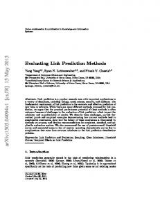
Figure 1: Packet Reception Rate (PRR), Received Signal Strength Indicator (RSSI) and Link Quality Indicator (LQI) variation of an intermediate link over a period of 2 hours.
15
20
0.6 0.4
R2=0.9386
0.2
PRR vs LQI Logistic Fit
0 50
60
70
80
90
100
110
120
LQI
(b) SNR
(c) LQI
Figure 2: Packet Reception Rate (PRR) as a function of Received Signal Strength Indicator (RSSI), Signal to Noise Ratio (SNR) and Link Quality Indicator (LQI) for 160 hours of data for 72 links. design is fundamentally different from STLE as we try to capture bursts of high quality periods using models trained with specific data traffic patterns instead of using heuristics. Link Quality Prediction: Applying data-driven methods on link quality prediction has been less studied. K. Farkas et al. [12] made link quality predictions using a pattern matching approach based on SNR. The main assumption is that the behavior of links shows some repetitive pattern. The authors suggest that the above assumption is valid for 802.11 wireless ad-hoc networks. Furthermore, they proposed XCoPred (using Cross-Correlation to Predict), a pattern matching based scheme to predict link quality variations in 802.11 mesh networks in [11]. 4C differs from XCoPred in several aspects: 4C combines both PRR and PHY parameters with prediction models trained off-line, whereas XCoPred considers SNR only and uses cross correlation without prior training. W. Yong et al. [25] used a decision tree classifier to facilitate the routing process. Their approach is to train the decision tree offline and then use the learned rules online. The results show machine learning can do significantly better where traditional rules of thumb fail. However, they only considered RSSI in their input features and overlooked other physical layer information, whereas our modeling explore much more parameters with different traffic patterns.
3. MODELING We propose to use machine learning methods to build models that predict the link quality with information from both physical layer and link layer. To predict the quality of the wireless links, we use a combination of the PHY parameters (RSSI, SNR and LQI) and the PRR filtered by a window mean estimator with exponentially weighted moving average (WMEWMA) [28]. The intuition behind our approach is quite simple. We supplement the WMEWMA estimator, accurate mainly for high and low quality links that are stable in nature, with physical layer information to improve the estimation for the intermediate quality links which are highly unstable and show the most variation. We first motivate our research with an exploratory analysis. Then, we formally define the problem trying to solve, the modeling methods, and the procedure of model training. The modeling results are presented in the end.
3.1
Exploratory Data Analysis
PHY information is a direct measurement of the wireless channel quality when a packet is received, so we should expect some level of correlation between PHY information and link quality. Figure 1 shows the PRR variation of a intermediate link over 120 minutes, as well as the corresponding RSSI and LQI variations in that period. The similar variation patterns suggest that we can leverage the PHY information to predict link quality. Indeed, there are routing protocols that operate based on LQI [1, 24]. However, due to the short temporal dynamics of wireless channel and differences in hardware calibration, it is hard to find well defined correlations between PHY information and PRR over different links and even different networks. We believe this is the reason why widely used routing protocols like CTP [14] often utilize PRR cost based link estimators. One question we would like to explore is to what extent we can correlate PHY parameters and PRR, such that we could use them as input in the prediction process of expected PRR. Figure 2 shows the relationships between PRR and the different PHY parameters. The curves were obtained with data collected as explained in Section 3.4. A simple visual inspection of Figures 2(b) and 2(c) shows that both LQI and SNR have a significant correlation with PRR. On the other hand, Figure 2(a) shows that RSSI has values spread over a wider range of PRR values for RSSI values in the −94 and −85 dBm range. The solid line shows the logistic fit for each of the curves. As expected, both LQI and SNR present very high R2 goodness of fit [6] values of 0.9386 and 0.8744 respectively. RSSI has a much lower R2 of 0.4348. Based on these results, there are a couple of observations we can make. First, our results agree with previous findings in [15] and [21] for SNR. However, our results extend the findings to LQI, and also show it is the PHY parameter that has the best goodness of fit. Second, our results for RSSI differ from those found in [23]. When collecting a larger number of experimental traces, we find that the LQI has a smaller variance than RSSI. We also noted that not all the links with −87 dBm RSSI values have PRR larger than 85%. In our data traces we get extreme cases of intermediate links with RSSI values larger than −87 dBm up to −74
dBm. Finally, based on our data analysis, it is clear that we should take advantage of PHY information to determine the expected packet reception. The following sections show how to use both PHY information and PRR to our advantage.
3.2 Problem Definition The model we want to create takes W packets as input to predict the reception probability of the next packet. In other words, the input to our model is a vector that is constructed from the the historical information of W packets. An input vector (Inputi ) is expressed as follows: Inputi = [P KTi−1 , P KTi−2 , . . . , P KTi−W ] and the output is the reception probability of the ith packet: P (Receptioni |Inputi ). The packet vector P KTi is comprised of packet reception rate and a subset of available physical layer information P HYi corresponding to a packet. It is written as: P KTi = [P RRi , P HYi ], P HYi ⊂ (RSSI, SN R, LQI)i All the values in a packet vector are discrete. P RRi is the WMEWMA output and has a range between [0, 1]. The physical parameters (RSSI, SNR and LQI) have different ranges ([−55, 45],[0, 50] and [40, 110] respectively), so we scale them down to the range [0, 1], such that the physical parameter vector P HYi is within the unit range of [0, 1]. With this notation, we can represent a lost packet as: P KTi = [P RRi , 0] where, P HYi = 0 since there is no physical parameter available for lost packets. In real world sensor network applications, the data traffic can be periodic (e.g. temperature monitoring) or aperiodic (e.g. event detection). We account for this behavior by using input vectors composed of data packets with fixed or random inter-packet interval (I) times. With a fixed I, the input vector is composed of periodic packets separated by the same time interval. For random I, we use a Bernoulli process to select packets such that the time intervals between two consecutive packets follow a binomial distribution whose mean equals to I. These two data composition methods enable our link prediction scheme to deal with varying periodicity of data as seen in real applications. We train models using different average I values and data composition methods to test the prediction performance under changing periodicity.
3.3 Prediction Methods The modeling method should satisfy the following requirements to be considered practical for sensor networks: – Small Training Data: The model should not need significant deployment efforts for gathering training data for extended periods of time. Otherwise, the overhead of gathering data to train the model alone might outweigh the benefits gained by using the model. – Light Weight Online Prediction: While training the model offline can be computationally costly, the implementation of the online link prediction scheme using the trained model should have low computational complexity and small memory requirements. Based on these guidelines, we tried three methods: Naive Bayes classifier (NB) is a simple probabilistic classifier based on Bayesian theorem with the conditional inde-
Parameters Input Feature Number of Links (L) Number of Packets (P ) Input Window (W ) Packet Interval (I)
Values P RR + {RSSI, SN R, LQI} 20, 7, 5, 3, 2, 1 36000, 10000, 5000, 1000, 500 1, 2, 3, 4, 5, 10 0.1, 0.2, 0.5, 1, 10, 60 (seconds)
Table 1: Tunable Parameters pendence assumptions: each feature in a given class is conditionally independent of every other feature. Although the independence assumption is quite strong and is often not applicable, NB works quite well in some complex real-world situations such as text classification [5]. Due to its simplicity, we consider NB advantageous in terms of computation speed and use it as a baseline of our comparison. Logistic Regression (LR) is a generalized linear model that predicts a discrete outcome from a set of input variables. It is an extensively used method in machine learning, and is easy to implement in sensor nodes. Artificial Neural Networks (ANN) is a non-linear modeling technique used for finding complex patterns in the underlying data. For modeling, we used a standard feedforward network with one hidden layer of 5 perceptrons. The small number of hidden units reduces the computational complexity for faster online prediction on a sensor node.
3.4
Data Collection
In order to train the model, we collected packet traces from two testbeds: a local wireless sensor network testbed and the Motelab [27], a sensor network testbed composed of 180 Tmote Sky motes. The local testbed is comprised of 54 Tmotes, installed on the ceiling of a corridor in a typical office building. We implemented a collection program to record the physical layer information of every received packet of a wireless link. During one data collection experiment, a sender node continuously transmits packets to a receiver node with 100 milliseconds inter-packet interval (Tx-power=0dB, channel 26). Upon packet reception, the receiver node records the sequence number, RSSI and LQI of the received packets. In addition, the receiver measures the noise floor level by sampling the environmental noise 15 times with 1 millisecond interval after every reception. The measurement of the noise floor level enables us to compute the SNR. We ran the data collection program on 68 sender-receiver pairs in different time slots to avoid inter-node interference. In total, we recorded information for approximately 5.4 million packets over 160 hours of data collection. Each of the 68 packet traces contains records for 80,000 packets. Among the 68 links, there are 12 low quality links (P RR < 10%), 14 intermediate links (10% < P RR < 90%), and 42 high quality links (P RR > 90%). For Motelab, we collected packet traces from 10 links for one hour. Different from the local testbed data, only RSSI and LQI was collected, and the inter-packet interval is set to 62.5 milliseconds (64 packets per second). As we show in Section 3.7, a dataset of this scale is more than enough to train prediction models with satisfying accuracy.
3.5
Tunable Parameters
We varied several parameters in the training process to explore the optimal training parameter collection. Table 1 shows the different parameter combinations with regards to the input data during the training of our models.
Model: LR
Model: ANN
0.4
0.4
0.3
0.3
0.3
0.2
0.2
0.1
0.1
0
0
1
2
3 5 Number of Links
7
20
MSE
0.4 MSE
MSE
Model: NB
0.2 0.1
1
2
3 5 Number of Links
7
0
20
1
2
3 5 Number of Links
7
20
Figure 3: Prediction errors for L = {1, 2, 3, 5, 7, 20}, P = 36000. Model: LR
Model: ANN
0.4
0.4
0.3
0.3
0.3
0.2
0.2
0.1
0.1
0
0
500
1000 5000 10000 36000 Number of Packets Per Link
MSE
0.4 MSE
MSE
Model: NB
0.2 0.1
500
1000 5000 10000 36000 Number of Packets Per Link
0
500
1000 5000 10000 36000 Number of Packets Per Link
Figure 4: Prediction errors for L = 5, P = {500, 1000, 5000, 10000, 36000}. We experimented with different input feature vectors as well as various W and I values during the training process. W denotes the amount the historical packets needed to make a prediction, whereas I decides the periodicity of the prediction. The choice of them can greatly affect the prediction quality and the feasibility of implementing the model on resource constrained sensor nodes. For the input feature, we tried combination of PRR with all the physical information (P RR + RSSI + SN R + LQI) as well as PRR with one of the parameters (P RR + RSSI/SN R/LQI). The input vectors are composed of data combined from a number of links (L) with a number of packets per link (P ). Ideally, the training data should cover links with different qualities such that the resulting model can cope with a large spectrum of link quality variation. To ensure maximum link diversity in terms of packet reception rate, we maximize the difference between the L links in the reception rate such that the average reception rates are evenly distributed from 0% to 100%. Hence, a larger L implies better link diversity in the training set. Note that although we only consider link diversity in the reception rate dimension, future work will explore this issue more deeply in a multi-dimensional space, where each dimension quantifies a different characteristic of the link, e.g., standard deviation and skewness. The number of packets (P ) used from each link is also a tunable parameter when training our models. From a practical point of view, for constructing the model using the proposed approach in a different environment, the users need to collect certain minimum amount (in terms of link diversity and length) of traces to replicate conditions from the target environment. We parameterize these constraints (L and P ) and explore the associated trade-off in the training process. To find a balance between the training data size and prediction accuracy, we vary the training dataset and compare the accuracy of the resulting model. We tried several combinations of link selection, ranging from using all the available links to selecting only one.
PRR Computation: Compute the PRR by applying the WMEWMA filter on the selected packets. To mimic the ETX calculation of 4Bit [13], we set the window size of the WMEWMA filter to 5 packets and α to 0.9. Input Vector Construction: Based on the input features, we take the PHY parameters of W packets and combine them with the most recent PRR value computed in the previous step to construct an input vector. We repeat this step until all selected packets are used. The target vector is also constructed during the process by checking the reception status of the next packet of each input vector: we mark the target (desired output) of an input vector as 1 if the next packet is received, and 0 otherwise. Model Training and Testing: Once the input vectors and the target are constructed, we randomly select 60% of the total input vectors as the training data and use the remaining 40% as the testing data. We train the three models with the training data and then apply the trained models to the testing data. The prediction results are compared with the corresponding target vector to assess the performance. The 4 steps described above will create, train and test all three models with the same parameter set in MATLAB. To avoid excessive training, we first run the procedure with fixed input features to narrow down the reasonable input data size (L and P ). We then fix the input data size and run the training procedure for different combinations of input features, W and I. Due to the simplicity of the NB and LR models, training for each model needs less than one minute on a regular PC. On the other hand, each training of the more complex ANN based models can take up to several hours. In the end, we repeat the procedure for more than 50 times using data from the local testbed and the Motelab testbed, resulting in more than 150 models trained with different parameter sets for each testbed. Although the number of models is large, their performance trend is relatively clear as discussed in the following sections.
3.6 Training Procedure
Here we discuss the performance of our three models when evaluated on the testing data. We plot the variation in the mean square error (MSE) as a function of input features, L, P , W and I. Based on the results, we propose the data requirement of training (L and P ) as well as the model selection guideline (W ) for the experimental evaluation in Section 5. Ideally, we would like to have the error as low as
Once the parameters are set, we use the following steps to train the models. Packet Selection: Select L links from the collected data. From each link, select P packets according to the I. As described in Section 3.2, the time intervals between packets can be either fixed or random based on the periodicity of I.
3.7
Modeling Results
Model: LR
Model: ANN
0.4
0.4
0.3
0.3
0.3
0.2
0.2
0.1
0.1
0
0
1
2
3 4 Window Size
5
10
MSE
0.4 MSE
MSE
Model: NB
0.2 0.1
1
2
3 4 Window Size
5
0
10
1
2
3 4 Window Size
5
10
Figure 5: Prediction errors for W = {1, 2, 3, 4, 5, 10}. Trained with L = 5, P = 1000. Model: NB P=5000
Model: LR P=10000
0.3
0.4
0.2 0
0
60
Model: ANN
P=5000
P=10000
0.2 0.1
0.2 0.5 1 10 Time Interval (Seconds)
P=1000
0.3
0.1 0.1
P=500
0.4 MSE
P=1000
MSE
MSE
0.4
P=500
P=500
P=1000
P=5000
P=10000
0.3 0.2 0.1
0.1
0.2 0.5 1 10 Time Interval (Seconds)
60
0
0.1
0.2 0.5 1 10 Time Interval (Seconds)
60
Figure 6: Prediction errors of I = {0.1, 0.2, 0.5, 1, 10, 60} seconds. Trained with L = 5, W = 1. possible when L, P and W are small and I is large. Note that although we trained models for the local testbed and the Motelab testbed respectively, their performance results are very similar and the overall trend is the same. As such, we only present the local testbed results for brevity. Input Features: Our results show that the choice of PHY parameters does not affect the prediction result much except for the NB models, so we omit the figure for brevity. Also, the LR and ANN models show better prediction capability than the NB models, which can be observed from the figures in this section. In the remainder of this section we show the modeling results of using P RR + LQI as the input feature. Number of Links (L): Figure 3 shows the variation in the prediction error of the three models as a function of L. Across all three models, we see a common trend of decreasing prediction error as L increases. For the NB models, the performance when using fewer links is much worse than for L = 20. However, for the LR and ANN models, the prediction error is small (≈ 0.2) if L ≥ 2. This shows that the performance for the LR and ANN models trained with only two or more links is comparable to the ones trained with multiple links. Hence, for modeling proposes, only a few links with intermediate PRR are required to model the variations in a large variety of links. Number of Packets per Link (P ): Next, we plot the variation in the prediction error of the models as a function of P . From Figure 4, we observe that for high values of P (36000), the prediction error of all three models is almost the same with P values as low as 5000. In fact, the prediction error increases significantly only after P is dropped below 1000. This shows that we only need around 1000 packets per link to train the prediction models. Window Size (W ): W corresponds to the amount of historical information required by the model to predict the reception probability of the next packet. Intuitively, large W means more information will be made available to the model, so it should improve the prediction performance at the cost of more buffering and processing needs. However, Figure 5 shows that the prediction error does not decrease very rapidly as we increase W from 1 to 10, which implies that only the most recent packet is important for the prediction. Therefore, the LR and ANN models should work reasonably well with a small window size such as W = 1. Inter Packet Interval (I): Intuitively, the longer the I,
the older is the packet reception information used by the model. Therefore, the prediction error should be worse because intermediate links may experience significant temporal dynamics. Figure 6 shows the prediction errors as the I (aperiodic) increases from 100 milliseconds to 1 minute, with the MSE of models trained with different P plotted together. It shows that prediction error does not degrade much until I = 1 minute, implying that our models are not sensitive to I < 1 minute when L = 5, P = 1000. Moreover, the MSE of models with different P shows that using higher P can reduce the prediction error. In our case, models trained with P = 5000 is enough to provide similar accuracy comparing to models with P = 36000. Periodic I gives similar results and are omitted here. Note that although shorter Is give better results, in practice a model trained with short I may not perform well when there is a mismatch between the I and real packet sending intervals. For example, a model trained with 1 second I assumes that the average data rate is 1 packet/second, and predicts the success probability of the next packet whenever a new packet is received. However, if the actual packet interval is 10 seconds, the prediction based on the 1 second interval assumption will expire for 9 seconds, and may not represent the success probability of the next packet. Therefore, a model performs the best when the actual packet interval matches the I value. A simple solution to this problem is to train multiple models with different I values and do best matching based on the data rate conditions seen in the field. We explore the same I mismatch issue in Section 5.3, and leave the full evaluation of the solution for future work. Summary: These results are quite significant. They essentially show that a user that wants to train a model just needs to gather several minutes (2-10 minutes) worth of data from only a few links (5-7 links) to reach an MSE that is similar to models trained with much higher number of links, and with significantly longer packet traces. Moreover, the trained model only need one historical packet for the prediction. We evaluate the statement experimentally in Section 5.
3.8
Performance Gain with Prediction
We also compare the prediction performance of our models with a Bernoulli process, an informed estimator based on the full knowledge of the link PRR ahead of time. We set the success probability of the Bernoulli process to be equal to
NB
LR
ANN
1
Bernoulli
Prediction Accuracy
Prediction Accuracy
1 0.8 0.6 0.4 0.2 0
0.11
0.21
0.44 0.69 0.76 Average PRR
0.83
LQI
PRR
LQI+PRR
Bernoulli
0.8 0.6 0.4 0.2 0
0.93
(a) Input feature = {LQI, P RR}, different models
0.11
0.21
0.44 0.69 0.76 Average PRR
0.83
0.93
(b) LR model with different input features
Figure 7: Prediction accuracy for links of varying PRR of models trained with L = 5, P = 5000, W = 1 and I = 10 seconds. the PRR, so the 1/0 trail generated by the Bernoulli process can be used to predict packet reception based on the overall link quality. We apply our models and the Bernoulli process on several empirical intermediate quality links and compare the prediction accuracy of different modeling methods and varying input features. The prediction accuracy is computed as the ratio of the correctly predicted packets to the total number of packets of the link. Figure 7(a) shows the performance of the NB, LR, ANN models and the Bernoulli process for wireless links of varying PRR. We see that for I = 10 seconds our prediction models consistently outperform the Bernoulli process. This result illustrates that our modeling approach can better adapt to link quality variations than the Bernoulli process. It also shows that LR based model can provide very good prediction accuracy at low computational costs. Figure 7(b) shows the prediction accuracy of LR models with different input features. In almost all cases, we see that the prediction models perform better than the Bernoulli process. Moreover, we see that the best prediction result is achieved by using both PRR and LQI in our input feature, followed by PRR and LQI only cases. We see that PRR does a better job than LQI, except for very good links on which the LQI based predictor performs better. The intuition behind this result is that although PRR is a good estimate for links with stable quality, it is too stable to account for the rapid quality variations. Additionally, LQI changes too drastically on wireless channel variations, making it unstable for long term estimations (unless the link is consistently good). By using the combination of LQI and PRR as input, the LR model can supplement the PRR with LQI, and therefore performs better in estimating link quality for intermediate links. Note that in some cases, the accuracy of Bernoulli process is even worse than the average PRR of the link. In essence, the packet losses/successes are often correlated [8] and therefore the underlying packet reception distribution is not a Bernoulli process. For example, suppose a 5-packet trace of the form 11110 is collected with P RR = 80%. A Bernoulli process with p = 0.8 will predict this sequence with prediction accuracy at least of 80% in only a 6 cases, namely 11110, 11111, 01110, 10110, 11010 and 11100. In all other 26 cases, the prediction accuracy will be < 60%, so the expected prediction accuracy (weighed over the likelihood of each sequence) will be less than the PRR value. This simple example shows the difficulties a link estimator faces: even if it captures the PRR correctly, the correct prediction is still not guaranteed.
4. ESTIMATOR DESIGN In this section we present the design of the 4C link estimator. We first show how we integrate the prediction based link
Figure 8: Overall Design of 4C. estimation with the existing link estimator, then discuss the main challenges and details of the model implementation.
4.1
Overview
4C shares a similar approach with the Short Term Link Estimator (STLE) [2]. It works in parallel with an existing link estimator, using information from overheard packets to predict the link quality of neighboring nodes. If 4C finds that it can provide a better path cost than the parent node of a sender, it will send beacon packets to the sender to announce itself a temporary parent as detailed in Section 4.3. After reception of this beacon, the sender will switch its next hop from the parent node designated by the routing protocol to the temporary parent. Thereafter, the sender will send future packets to the temporary parent until the number of consecutive lost packets exceeds a threshold, or the temporary parent denounce itself. In this case, the sender node will switch back to the old parent node. In essence, both STLE and 4C attempt to reduce the total number of transmissions per packet by using temporary routes on the basis of a stable network topology established by the routing protocol such as CTP. However, there are two main differences between STLE and 4C. First, they apply to different traffic patterns. 4C is focused on providing a more informed link estimation whereas the main goal of STLE is to detect short term reliability of intermediate links using a simple heuristic procedure: 3 consecutive packet receptions means the link is usable, and a loss means the links is no longer usable. On the other hand, 4C can fit to a wide range of traffic patterns by utilizing appropriate models. For example, experimental results in Section 5 show that with the logistic regression model, 4C works the best when tested using similar traffic patterns used for training. On the other hand, STLE is most suited for bursty link discovery, therefore its heuristic-based approach applies specifically to only a bursty traffic pattern. Second, STLE is mainly a qualitative measurement whereas 4C is quantitative in nature. STLE can identify whether an intermediate link reliable or not, but it can not specify how reliable the intermediate link is. In contrast, 4C is designed to give a quantitative estimation of the link quality.
4.2 Overall Design Figure 8 presents the overall design of the 4C. In general, 4C operates in the intercept (overhearing) nodes and interacts with all three core components in CTP: the forwarding engine, which handles data packet sending and forwarding, the routing engine, which is in charge of choosing the next hop (parent) based on the link estimation as well as processing network-level information such as congestion detection, and the link estimator that is responsible for estimating the quality of the links to single-hop neighbors. 4C works in two stages: link prediction and path evaluation. In link prediction, 4C uses the data packet overheard by the forwarding engine and ETX from the link estimator to estimate the link quality of neighboring nodes. When the forwarding engine overhears a packet from a node, it passes the packet to 4C. 4C records the packet information, i.e., sequence number, packet sender and PHY parameters in its neighbor table. Then, 4C queries the link estimator for the link ETX of the sender, and takes the reciprocal of the returned ETX to get the estimated PRR. Finally, the underlying prediction model takes the estimated PRR and the PHY parameters as the input and outputs a reception probability for the next packet. In the path evaluation stage, 4C uses the predicted reception probability to evaluate the path cost for the sender assuming the intercept node is the sender’s parent. This is done by adding the path cost of the intercept node itself with the reciprocal of the predicted reception probability. If the calculated path cost is smaller than the actual path cost of the sender by a threshold, 4C sends beacons to the sender, announcing itself to be the temporary parent. 4C sets the threshold adaptively so that the additional overhead introduced by the announcement beacon will not offset the potential gain of using the temporary parent. The temporary parent announcement process is discussed in Section 4.3. On the sender side, after receiving the announcement beacon, 4C notifies the forwarding engine about the temporary parent. The sender then starts forwarding its traffic to the temporary parent. The temporary parent continues to be the sender’s next hop until one of the following three events happens: temporary parent denounces its parent status, the routing engine assigns a new parent, or the number of consecutive packet losses exceeds a threshold. If any of the above three cases occurs, the sender will switch back to the parent designated by the routing engine. An important design decision is which prediction method 4C should use. To implement a prediction model on conventional sensor network hardware, we need to select a model that is the most suitable for online link prediction. While the NB based model is the fastest, it has the worst performance out of the three approaches. The LR and ANN based models are even in performance, but the ANN model has computational complexity several orders of magnitude higher than the LR model. Hence, we decide to favor the LR model for implementation on sensor nodes.
4.3 Temporary Parent Announcement A question we need to explore is when should a node announce to be a temporary parent such that the overhead of announcement beacons will not offset the cost gain. To investigate the problem, let’s assume the following scenario. Since a routing gradient has already been established by CTP, each node should have an associated path cost, which
denotes the number of transmissions needed to deliver one packet to the root node. We define the path cost of a sender node S as CS , and the path cost of the sender’s parent, P , as CP . Similarly, we define the cost of sending a packet on the link S → P as CS→P . Let’s assume the packets sent by S are overheard by node T . T decides to be the temporary parent of S, so it needs to send beacons to notify S. In order to guarantee the reception of the notification, T needs to send CT →S beacons to the sender on average. Moreover, another CT →S beacons are needed when T decides to renounce its temporary parent status. Together, we note the cost of sending notification beacons as Cbeacon = 2 × CT →S . Suppose the temporary parent T forwards n data packets for S during the process. The potential cost gain will be: GAIN = n × ((CP + CS→P ) − (CT + CS→T )) − Cbeacon The gain should be greater than 0, so we have n × ((CP + CS→P ) − (CT + CS→T )) − Cbeacon > 0, which transforms to CP + CS→P > CT + CS→T +
2 × CT →S . n
(1)
Formula (1) can be viewed as the criteria for intercept nodes to announce the status of temporary parents. If it is satisfied, an announcement of temporary parent will be beneficial even counting the beacon overhead. An important parameter here is n, the number of packets that will be forwarded by the temporary parent. In our implementation, we take a conservative stance and set n = 1. In this case, as long as the sender sends more than one packet to the temporary parent, the overall cost will be further reduced.
4.4
Implementation Issues
A critical issue is the computation speed of the prediction module. A logistic regression classifier, if implemented naively, requires a vector multiplication and sigmoid function to compute the predicted reception probability for the next packet. In the resource constrained sensor networks, it is not feasible to do this natively in terms of computational cost. Furthermore, 4C is a part of the network stack, which normally demands agile response to network events. As such, prediction speed is one of the main concerns of the model implementation. 4C uses PLAN, a pairwise linear approximation proposed by H. Amin et al. [3] to implement the sigmoid function. PLAN approximates the sigmoid function with 5 line segments and requires only one bit shift and addition operation to compute a sigmoid. In addition, optimizations are made to avoid the use of floating point operations. Our implementation running on a Tmote Sky mote requires 0.5 ± 0.004 milliseconds to compute a prediction, well within the time constraints of the networking processing stack in TinyOS. In addition to speed, another issue is the extendibility of the prediction module. By design, the prediction module is implemented with a generic interface, so that the module can be replaced by other models as long as the input is the same. The LR prediction module accepts the coefficients from a LR model as its parameter, so it can be easily extended to use different LR models by changing the coefficients. In our experiments, we used several LR models trained with different parameters as discussed in Section 5.
V1
V2
D1 D2 Node Pairs
H1
H2
(a) Motelab
6 Avg. Delivery Cost
6
4C STLE 4Bit
Avg. Delivery Cost
Avg. Delivery Cost
9 8 7 6 5 4 3 2 1 0
5 4 3 2 1 0
51−0
48−0 Node Pairs
5 4 3 2 1 0
45−0
(b) Local – Different Nodes
0.1
0.2 0.5 1 10 Sending Interval (Second)
(c) Local – Different Intervals
Figure 9: Cost comparison of 4C, STLE and 4Bit. Actual node pairs in (a) are listed in Table 2. There are also stability issues to consider. A practical problem occurs when CTP selects a new parent due to link quality variations of the neighboring nodes, the path cost change need some time to propagate. In this routing information propagation stage, 4C should not announce any temporary parent because the routing gradient of the network will likely be changed. To avoid this situation, we added some hysteresis to the process. We use a counter to suppress temporary parent announcements: if a parent change from the routing engine is detected, it will stop forwarding packets to the temporary parent immediately, and set the suppression counter to a preset value H. The counter value will decrease by 1 after each packet is sent to the new parent until it reaches 0. While the counter is not 0, 4C will not send any temporary parent announcement. In other words, 4C will not operate after a parent change until H packets are sent to the new parent. In our experimental evaluation, we set the H value to 3. To avoid excessive retransmission, we also set an additional threshold to the maximum number of packet losses when forwarding packets to a temporary parent. This was implemented to avoid a broken link situation. If the link from a sender to its temporary parent is broken, the temporary parent will not be able to denounce itself. In this case, if the forwarding engine is using a temporary parent, it will switch back to the old parent after 5 packets are lost.
5. EXPERIMENTAL RESULTS 5.1 Experimental Setup Our experimental evaluation can be divided in two stages. In the first stage, we run single sender experiments to compare the performance of 4C, STLE [2] and 4Bit [13] under the similar experimental settings used by the authors of STLE. In the second stage, we further extend the evaluation of 4C under more realistic settings with multiple sender experiments, in which all nodes in the network send packets to the root node periodically. Because the multiple sender experiments better emulate typical WSN traffic pattern than the single sender experiments, we believe the multiple sender experiments can provide us more thorough evaluation in terms of delivery cost. The detailed experimental settings and results are discussed in the following sections. We conducted experiments on the Motelab testbed, our local indoor 54 node testbed and a 21-node outdoor testbed. For all local testbed and outdoor experiments, we set the radio output power level of CC2420 to −25dB, packet length to 30 bytes and use wireless channel 26 to avoid 802.11 interference. For the Motelab experiments, the parameters are the same except for the radio output power is set to max (0dB) for better connectivity.
Label V1 V2 D1 D2 H1 H2
Node Pair 183 → 50 137 → 9 183 → 9 137 → 50 9 → 50 183 → 137
Description Vertical Vertical Diagonal Diagonal Horizontal Horizontal
Table 2: Node pairs in the Motelab experiments.
5.2
Single Sender Experiment Results
Due to the similarity of STLE and 4C design, it is reasonable to compare the performance of these two link estimators. To provide a plausible comparison, we implemented the STLE based on the design of Alizai et al. [2] to the best of our ability 1 . We followed the experimental settings in [2] and conducted a series of single sender experiments in both Motelab and the local testbed. In single sender experiments, only the sender node sends packets to the root node with a fixed interval using CTP. In each experiment, we keep the same sender/root pair but employ different link estimators to compare the communication costs of CTP with 4C, STLE and 4Bit under the same network condition. We vary the node pairs and packet sending interval (SI) to study how these link estimators perform under varying conditions. Please note that SI is different from the inter-packet interval (I) used in model training: SI represents the data rate in the application layer, whereas I is a parameter used in the training. We use the average delivery cost as the performance parameter, which refers to the number of communications needed to deliver a packet to the sink. It is the sum of the send attempts including retransmissions, at each hop along the path. Figure 9 illustrates results from these experiments. Motelab Experiments: To emulate the network environment of the original STLE experiments as close as possible, we used three of the node configurations selected in [2]: vertical, diagonal and horizontal. Vertical configuration means the source and destination are on different floors and on the same end; diagonal configuration means the source and destination are on different floors but on the opposite ends; and in the horizontal configurations the source and destination are on the same floor and on the opposite ends. The actual node pairs used are listed in Table 2. For each node pair, we let the source node send packets with SI = 200 milliseconds for 15 minutes using 4C, STLE and 4Bit. 4C uses an LR model trained with data collected form the Motelab using the following parameters: input features = P RR + LQI, L = 5, P = 1000, W = 1 and fixed I = 200 milliseconds. Figure 9(a) shows the average delivery costs of the Motelab experiments. In the vertical configurations, the costs 1 We tried getting the STLE code a few times from the Feb. to Aug. 2010, but the code was never provided by the authors.
4C STLE 4Bit
3.1% 2.5% 18.0% 46.1% 17.5% −0.9% 2.2% 12.2% 11.7% 3.2% 19.0% −1.7%
10L
10H
30L
30H
60L
Avg. Delivery Cost
Avg. Delivery Cost
8 7 6 5 4 3 2 1 0
60H
8 7 6 5 4 3 2 1 0
33.3% 25.2%
10L
32.0% 16.6%
10H
8 7 6 5 4 3 2 1 0
3
31.3%
27.2% 7.6% 22.6% 7.2% −2.0% −4.3% 24.9% −5.5% −0.5%
10L
10H
30L
30H
0.9% 8.2% −0.9% 1.8%
30L
30H
60L
9.3% 4.8%
60H
(b) Local, M2
60L
20.8% 2.8%
60H
Avg. Delivery Cost
Avg. Delivery Cost
(a) Local, M1
2.5% 1.7%
4C 4Bit
14.2%
10.8%
M1
M2
2
1
0
(c) Local, M3
(d) Outdoor, M1 and M2
Figure 10: Cost comparison of multiple sender experiments run on the local testbed and the outdoor testbed. Y axis denotes the average delivery cost (lower is better). Labels in the x axis in figure (a), (b) and (c) note the experiment conditions: the number 10, 30 or 60 is the sending interval, and the letter L, or H represents the network density. The gray boxes on top of the bars represent the beacon overhead, and the percentages on the top indicate the reduction rates of 4C over STLE and/or 4Bit. of all three link estimators are similar due to the short distance between the source and destination in terms of routing. However, STLE may have a larger cost as it can be seen in the V1 case. In the diagonal cases, both STLE and 4C outperform 4Bit. Finally, in the horizontal cases, usually the most common case of nodes on the same horizontal plane for many applications, 4C clearly outperforms both STLE and 4Bit. STLE may provide better performance compared with 4Bit in some cases (H1), or comparable in some other cases (H2). It is clear that overall, the original CTP with 4Bit has higher delivery costs comparing with STLE and 4C. The results show in the most common cases for real deployments (horizontal), 4C can perform significantly better than STLE. In the vertical and diagonal cases, its performance is at least comparable to STLE. Local Testbed Experiments: We repeat the single sender experiments with three node pairs in the local testbed to verify the results. Also, to test the effect of packet sending interval, we vary the SI from 100 milliseconds to 10 seconds. In all these experiments, 4C always employs the prediction model trained with a I that matches the actual SI. Figure 9(b) presents the cost comparison between CTP with 4C, STLE and 4Bit link estimator run on three node pairs. Due to the topological constrains of the testbed, all the node pairs are of horizontal configuration. The result is similar to the horizontal experiment results from Motelab: either 4Bit or STLE have the highest cost, whereas 4C has the lowest cost in all the experiments. Furthermore, Figure 9(c) shows that with varying data rates, 4C outperforms STLE and 4Bit in all our experiments. These results lead us to believe that overall, 4C can harness the potential of intermediate links better than STLE does under different network environments and varying traffic rates. Even in the worse performance cases, the delivery cost of 4C is still comparable with that of STLE or 4Bit.
5.3 Multiple Sender Experiment Results We continue our evaluation using multiple sender experi-
Model M1 M2 M3
L 5 5 5
P 1000 1000 5000
W 1 1 1
I 10 seconds, periodic 10 seconds, aperiodic 60 seconds, aperiodic
Table 3: Model parameters used in the experiments. ments, which try to emulate the traffic pattern of a typical data collection application where all the nodes in the network send packets to a single root node. Similar to the single sender experiments, the nodes send packets for one hour, using CTP with 4C, STLE and 4Bit respectively in each experiment. Furthermore, we repeat every experiments three times to minimize the effects of temporary network irregularities. Due to the relatively low data rate in many WSNs applications, we focus on communication costs and reliability, and leave latency and throughput for future work. We vary network density and packet sending interval (SI) in these experiments. Network density refers the the number of nodes we include in each experiment. In the local testbed experiments, we used two densities: high density, which includes all the 54 nodes in the testbed, and low density, which includes 18 nodes in a line topology. For SI, we use 10, 30 and 60 seconds in the local testbed, and 10 seconds in the outdoor testbed. The sending intervals are longer than what we used in the one sender experiments because i) traffic rates in these intervals are more aligned with some real WSN applications, and ii) longer intervals can reduce network congestion given the larger number of senders. Moreover, to avoid correlated interferences, the actual packet sending interval is randomly chosen from [ 12 SI, 23 SI]. To evaluate the performance of models trained with different parameters, we use three LR models based on the modeling results discussed in Section 3.7. As seen in Figure 6, LR models trained with L = 5, P = 1000 are enough to provide good prediction results when I = 10 seconds, whereas models trained with L = 5, P = 5000 perform well when I = 60 seconds. So, the first two models we chose (M1 and M2) are trained with input features = P RR + LQI,
L = 5, P = 1000, W = 1, periodic and aperiodic I = 10 seconds. The third one (M3) has the same parameters as M2 except for P = 5000 and the aperiodic I = 60 seconds. The model parameters are listed in Table 3. In the outdoor testbed, we repeat our experiments to verify the results. Model M1 and M2 are used, and the SI is 10 seconds. The network density is fixed to 21 nodes. All other parameters are the same as local testbed experiments. Unfortunately, we could not verify our results in the Motelab testbed with multiple senders due to time constrains. Figure 10(a), 10(b) and 10(c) compare the delivery costs of the local testbed experiments. In each figure, the labels in the x axis note the experiment conditions: the number 10, 30 or 60 represents the SI, and the letter L or H represents the network density (18 and 54 nodes respectively). The gray boxes on top of the bars represent the beacon overhead, i.e., the number of beacons sent per data packet delivered. The percentages on the top of the bars are the reduction ratio of 4C compared to STLE and 4Bit results. Next, we discuss the results in terms of delivery cost and beacon overhead. Delivery cost refers to the number of send attempts needed to deliver a packet to the sink. From Figure 10(a), a significant cost reduction of 4C over 4Bit (more than 46%) can be observed on the experiments with 10 seconds SI. Since the LR model (M1) used in 4C is also trained with I = 10 seconds, this reduction gain implies that the 4C is indeed selecting better routes comparing with 4Bit. The cost reduction is less significant as the SI increases, but the cost of 4C is still comparable with STLE and 4Bit even in the worst case. On other hand, STLE generally shows lower cost than 4Bit, but 4C is able to outperform STLE in almost all cases. Similar gain can be observed in Figure 10(b). In Figure 10(c), which shows the results of 4C using model trained with I = 60 seconds, we see that cost gain is more pronounced in high SI scenarios, i.e., SI = 30 and 60, than SI = 10 seconds cases. This indicates that the training parameters of the model indeed affect the prediction performance: the models trained with I = 10 seconds can do well under the same network traffic rate, but when the traffic pattern and I are misaligned, the model can not effectively predict the packet reception probability anymore. However, even in these cases the performance of 4C is comparable to 4Bit, the default link estimator of CTP. Our outdoor experiment confirmed this observation. In Figure 10(d) we observe that 4C shows more than 10% improvement over 4Bit in terms of average delivery cost. Beacon Overhead is the average number of beacons sent by the routing protocol while it delivers one packet to the sink. The number of beacons represents the overhead of the routing protocol for maintaining a routable network structure. Figure 10 show that beacon overheads (depicted as gray box on top) of 4C, STLE and 4Bit are similar in almost all experiments, which indicates that 4C does not incur significant overhead comparing to the CTP with 4Bit.
6. DISCUSSION Advantages of a Data-Driven Approach: According to the communication theory, the PRR-SNR correlation can be derived from the frame size, the coding scheme and the bit error rate defined by the modulation format [19]. For example, the link layer models proposed in [32] provide deterministic functions to calculate PRR with SNR for a variety of modulation formats and coding schemes. Although
these models are useful in network simulation, this idealized approach can not provide accurate PRR estimation for intermediate quality links which show large PRR variance [30, 15]. Moreover, research [7, 31, 21] shows that the actual correlation between PRR and PHY parameters may be different due to hardware specific variations. As shown by Son et al. [21], even at the same measured signal strength at the receiver, the signals from different sources may have different levels of distortion, in turn affecting the packet reception differently. Therefore, in order to find the right function to calculate PRR based on SNR, a user will need to collect PRR/SNR data across all possible node pairs in a network, and the function coefficients for each node pair may be different. This level of complexity will render this approach infeasible for any network with more than dozens of nodes. We account for this problem with the data driven approach. With a sufficient large training dataset collected from actual links in the network, the machine learning algorithms can find the optimal function by minimizing the error between the output and the actual packet reception. From a modeling perspective, this approach can be viewed as a way to find the best overall correlation between PRR and PHY parameters given a training dataset, whereas the communication theory approach is a way to find the best correlation for a node pair. Therefore, the trained models can represent the optimal correlation over the underlying network as a whole. In addition, our model combines the PRR and a variety of PHY parameters to estimate the link quality instead of using only SNR. Another difference is that the 4C employs a receiver-initiated design, which means the quality estimation happens on the receiver side. Training Data Requirements: A major concern of a data driven approach is the data requirement. In the previous sections we show that our modeling approach can indeed capture the underlying PRR distribution with small amount of data. The performance improvement when modeling parameters and actual conditions matched, implies that there are some repeatable patterns in packet reception. Therefore, a sufficiently large training set is necessary to capture the underlying PRR distribution. Both the simulation and experimental results show that a training set consisting of packet reception data collected from a few links for several minutes is sufficient to train the prediction model. If sufficient training data is available, our model can find correlations that exceed the hundred of milliseconds, and extend to many tens of seconds as shown in our results in Section 5. Limitations: The evaluation results show that the performance of prediction models is similar with state-of-art link estimator when there are non-negligible network dynamics, e.g. changing packet sending interval. As discussed in Section 5, 4C performs on par with 4Bit when the actual traffic pattern does not match the modeling parameter, indicating that the prediction is inaccurate in this case. This is due to the fact that 4C only incorporates one prediction model, and consequently, can not adapt to varying network conditions from the original training set very well. However, we showed that the training can be done with a small amount of data, and 4C could potentially use multiple models trained with freshly collected data for different network conditions. Furthermore, it is possible to apply online learning algorithms in 4C such that the prediction model can evolve with the changing network conditions. We leave task of examining the 4C performance with other network dynamics, such as
varying radio power and packet size, to future work.
7. CONCLUSIONS In this paper we showed the usefulness of link quality prediction based on different machine learning methods, such as, naive Bayes classifier, logistic regression and artificial neural networks. Our models take a combination of PRR and PHY information as input, and output the reception probability of the next packet. We showed that users need very little data (5-7 links for a couple of minutes) in order to train the models in the environments tested. Our analysis showed that logistic regression works well among the three models with the additional advantage of having the small computational cost. Using this knowledge, we implemented 4C, a novel link quality estimator in TinyOS. We conducted extensive experiments in the Motelab and our local indoor testbeds, as well as an outdoor deployment. Our results show improvements in the order of 20% to 30% compared with 4Bit and STLE estimators in single and multiple sender experiments, with some cases improving performance by more than 45%. Future research directions involve incorporating time information to the existing input vector to help the model adapt better to varying traffic patterns and the use of online learning algorithms for link quality prediction under dynamic conditions.
8. ACKNOWLEDGEMENTS Special thanks to Ankur Kamthe for providing data traces for the Motelab testbed and valuable discussions on 4C design, Varick Erickson for helping in the outdoor testbed, the anonymous reviewers for their insightful feedback, and Carlo Fischione for shepherding this paper. This material is based upon work partially supported by the National Science Foundation under grant #0923586, the California Institute for Energy and Environment under grant #MUC-09-03, and the Center for Information Technology Research in the Interest of Society under grant #442130-19900.
9. REFERENCES [1] MultiHopLQI, TinyOS 1.x. ´ [2] M. H. Alizai, O. Landsiedel, J. Agila Bitsch Link, S. G¨ otz, and K. Wehrle. Bursty traffic over bursty links. In SenSys ’09, pages 71–84. ACM, 2009. [3] H. Amin, K. M. Curtis, and B. R. Hayes-Gill. Piecewise linear approximation applied to nonlinear function of a neural network. IEE Proceedings - Circuits, Devices and Systems, 144(6):313–317, 1997. [4] N. Baccour, A. Koubˆ a, H. Youssef, M. Ben Jamˆ aa, D. do Ros´ ario, M. Alves, and L. Becker. F-lqe: A fuzzy link quality estimator for wireless sensor networks. In EWSN ’10, volume 5970 of Lecture Notes in Computer Science, pages 240–255. Springer Berlin / Heidelberg, 2010. [5] C. M. Bishop. Pattern Recognition and Machine Learning. Springer, 2006. [6] G. Casella and R. L. Berger. Statistical Inference. Duxbury Press, 2001. [7] A. Cerpa, N. Busek, and D. Estrin. SCALE: A tool for simple connectivity assessment in lossy environments. Technical Report 0021, UCLA, 2003. [8] A. Cerpa, J. Wong, L. Kuang, M. Potkonjak, and D. Estrin. Statistical model of lossy links in wireless sensor networks. In IPSN ’05, pages 81–88, 2005. [9] A. Cerpa, J. Wong, M. Potkonjak, and D. Estrin. Temporal properties of low power wireless links: Modeling and implications on multi-hop routing. In MobiHoc ’05, pages 414–425. ACM, 2005.
[10] D. S. J. De Couto, D. Aguayo, J. Bicket, and R. Morris. A high-throughput path metric for multi-hop wireless routing. In MobiCom ’03, pages 134–146. ACM, 2003. [11] K. Farkas, T. Hossmann, F. Legendre, B. Plattner, and S. K. Das. Link quality prediction in mesh networks. Computer Communications, 31(8):1497–1512, 2008. [12] K. Farkas, T. Hossmann, L. Ruf, and B. Plattner. Pattern matching based link quality prediction in wireless mobile ad hoc networks. In MSWiM ’06, pages 239–246. ACM, 2006. [13] R. Fonseca, O. Gnawali, K. Jamieson, and P. Levis. Fourbit wireless link estimation. In HotNets VI. ACM, 2007. [14] O. Gnawali, R. Fonseca, K. Jamieson, D. Moss, and P. Levis. Collection tree protocol. In SenSys ’09, pages 1–14. ACM, 2009. [15] D. Lai, A. Manjeshwar, F. Herrmann, E. Uysal-Biyikoglu, and A. Keshavarzian. Measurement and characterization of link quality metrics in energy constrained wireless sensor networks. In GLOBECOM ’03, pages 446–452, 2003. [16] P. Levis, S. Madden, J. Polastre, R. Szewczyk, K. Whitehouse, A. Woo, D. Gay, J. Hill, M. Welsh, E. Brewer, and D. Culler. TinyOS: An operating system for sensor networks. In Ambient Intelligence, pages 115–148. Springer Berlin Heidelberg, 2005. [17] J. Polastre, R. Szewczyk, A. Mainwaring, D. Culler, and J. Anderson. Analysis of wireless sensor networks for habitat monitoring. pages 399–423, 2004. [18] G. J. Pottie and W. J. Kaiser. Wireless integrated network sensors. Commun. ACM, 43(5):51–58, 2000. [19] T. Rappaport. Wireless Communications: Principles and Practice. Prentice Hall PTR, 2001. [20] M. Senel, K. Chintalapudi, D. Lal, A. Keshavarzian, and E. J. Coyle. A kalman filter based link quality estimation scheme for wireless sensor networks. In GLOBECOM ’07, pages 875–880. IEEE, 2007. [21] D. Son, B. Krishnamachari, and J. Heidemann. Experimental study of concurrent transmission in wireless sensor networks. In SenSys ’06, pages 237–250. ACM, 2006. [22] K. Srinivasan, M. A. Kazandjieva, S. Agarwal, and P. Levis. The β-factor: measuring wireless link burstiness. In SenSys ’08, pages 29–42. ACM, 2008. [23] K. Srinivasan and P. Levis. RSSI is under appreciated. In EmNets ’06, 2006. [24] G. Tolle and D. Culler. Design of an applicationcooperative management system for wireless sensor networks. In EWSN ’05, pages 121–132, 2005. [25] Y. Wang, M. Martonosi, and L. Peh. Predicting link quality using supervised learning in wireless sensor networks. ACM SIGMOBILE Mobile Computing and Communications Review, 11(3):71–83, 2007. [26] G. Werner-Allen, K. Lorincz, J. Johnson, J. Lees, and M. Welsh. Fidelity and yield in a volcano monitoring sensor network. In OSDI ’06, pages 381–396. USENIX, 2006. [27] G. Werner-Allen, P. Swieskowski, and M. Welsh. Motelab: a wireless sensor network testbed. In IPSN ’05, page 68. IEEE, 2005. [28] A. Woo, T. Tong, and D. Culler. Taming the underlying challenges of reliable multihop routing in sensor networks. In SenSys ’03, pages 14–27. ACM, 2003. [29] N. Xu, S. Rangwala, K. K. Chintalapudi, D. Ganesan, A. Broad, R. Govindan, and D. Estrin. A wireless sensor network for structural monitoring. In SenSys ’04, pages 13–24. ACM, 2004. [30] J. Zhao and R. Govindan. Understanding packet delivery performance in dense wireless sensor networks. In SenSys ’03, pages 1–13. ACM, 2003. [31] G. Zhou, T. He, S. Krishnamurthy, and J. A. Stankovic. Impact of radio irregularity on wireless sensor networks. In MobiSys ’04, pages 125–138. ACM, 2004. [32] M. Zuniga and B. Krishnamachari. Analyzing the transitional region in low power wireless links. In SECON ’04, pages 517–526. IEEE, 2004.