A BAYESIAN APPROACH FOR BLIND SEPARATION OF ... - CiteSeerX

A BAYESIAN APPROACH FOR BLIND SEPARATION OF SPARSE SOURCES C. Févotte and S. J. Godsill CUED/F-INFENG/TR.511 January 2005

University of Cambridge Department of Engineering Trumpington Street Cambridge CB2 1PZ United Kingdom Email: {cf269,sjg}@eng.cam.ac.uk

´ FEVOTTE AND GODSILL: A BAYESIAN APPROACH FOR BLIND SEPARATION OF SPARSE SOURCES

1

Abstract We present a Bayesian approach for blind separation of linear instantaneous mixtures of sources having a sparse representation in a given basis. The distributions of the coefficients of the sources in the basis are modeled by a Student t distribution, which can be expressed as a Scale Mixture of Gaussians, and a Gibbs sampler is derived to estimate the sources, the mixing matrix, the input noise variance and also the hyperparameters of the Student t distributions. The method allows for separation of underdetermined (more sources than sensors) noisy mixtures. Results are presented with audio signals using a Modified Discrete Cosine Transfrom basis and compared with a finite mixture of Gaussians prior approach. These results show the improved sound quality obtained with the Student t prior and the better robustness to mixing matrices close to singularity of the Markov Chains Monte Carlo approach.

Index Terms Blind Source Separation, Independent Component Analysis, Sparse Representations, Bayesian Estimation, Markov Chains Monte Carlo methods.

I. I NTRODUCTION Blind Source Separation (BSS) consists in estimating n signals (the sources) from the sole observation of m mixtures of them (the observations). In this paper we consider linear instantaneous mixtures of time series: at each time index, the observations are a linear combination of the sources at the same time index. (Over)determined (m ≥ n) non-noisy linear instantaneous mixtures have been widely studied, within the field of Independent Component Analysis (ICA), assuming independent and identically distributed (i.i.d) sources and using higher order statistics (see [1], [2] for a survey), or using correlation (e.g, [3]), non-stationarity (e.g, [4]), or both (e.g, [5]), leading to second order statistics based methods. These methods require at least mutual decorrelation of the sources (strict independence being required by high order statistics based methods) and little prior information on each source (typically, the sign of the kurtosis or mild hypotheses on spectra). These methods have proved to perform well, and one can reasonably argue that there is little left to be done in separation of (over)determined non-noisy linear instantaneous mixtures. Difficulties arise when dealing with mixtures which are possibly underdetermined and possibly noisy. The underdetermined case in particular is very challenging because contrary to (over)determined mixtures, estimating the mixing system is not sufficient for reconstruction of the sources, since for m < n the mixing matrix is not invertible. Then, it appears that separation of underdetermined mixtures requires important prior information on the sources to allow their reconstruction. Prior information can also be helpful for reconstructing the sources in noisy environments. In this paper, we propose to tackle the general linear instantaneous model (possibly underdetermined, possibly noisy) using the assumption of sparsity of the sources on a given basis. This assumption means that only a few coefficients of the decomposition of the sources on the basis are significantly non-zero. The use of sparsity to handle the general linear instantaneous model, has arisen in several papers in the areas of learning [6]–[8] and January 21, 2005

DRAFT

2

TECHNICAL REPORT OF CUED

source separation [9]–[13]. In the source separation context, source time series can be assumed to be sparse in time (speech sequences with silences are considered in [9], which describes a source separation method adapted from the learning method in [7]) but more generally to have a sparse representation on a given dictionary, possibly overcomplete (number of elements of the dictionary greater than the length of the signals). The aim of these methods then becomes the estimation of the coefficients of the sources in the dictionary and not the time series themselves. The time series are then reconstructed from the estimated coefficients. Besides the methods in [12], [13] which rely directly on disjoint time-frequency supports of the sources and propose deterministic methods, the methods in [6]–[11] model the distributions of the coefficients of the sources (the priors) with a distribution gathering most of its probability around zero and presenting heavy tails, thus modelling sparsity. The methods then proceed in two steps: the first one consists in learning the mixing matrix from the data, the second one in inferring the sources from the learnt mixing matrix and the data, with respect to the chosen prior on the sources 1 . In [7]–[10], the coefficients of the sources are given a Laplacian prior. Learning is performed via clustering in the mixtures space in [10] and via a Maximum Likelihood (ML) approach in [7]–[9]. The latter approach requires marginalization of the sources in the likelihood expression, which is done via a Laplacian approximation of the integral in [7], [9] and via a variational approximation of the Laplacian prior in [8]. Inferring is realised by linear programming in [7], [9], [10] while obtained as a by-product of the EM optimisation procedure used in [8]. In [6], [11], the coefficients of the sources are given a Finite Mixture of Gaussians (FMoG) prior distribution with 2 or 3 states (one state “off” corresponding to a Gaussian with very small variance, possibly zero, and high probability, one or two state(s) “on” corresponding to Gaussians with big variance and small probability). In [6], learning is achieved via a full ML optimisation, which is easily done taking advantage of the source coefficients being Gaussian conditionally upon the states. Inferring the sources requires inferring the states, which is done by a Gibbs sampling step. A pseudo-ML criterion is used for learning in [11] by truncating the full ML criterion to its n+1 dominant terms, which is equivalent to the assumption that only one source can be “on” at each time-frequency point. Inferring of the sources is then done by marginalisation over the all the possible states. The authors of [11] present results with speech signals decomposed on a MDCT orthonormal basis [14]. The method proves to perform as well as the full ML criterion approach (with decreased computational burden) and better than [7] in the presence of noise. The use of a basis provides equivalence between representations in the time domain and transform domain, and separation can be simply performed in the transform domain instead of the time domain. The use of an overcomplete dictionary is appealing because it allows potentially sparser representations but is less straightforward than the use of a basis because of the one-to-many mapping between the time and transform domains [10]. Motivated by the results of Student t modeling for sparse Bayesian learning [15], [16], we consider a Student t prior on the source coefficients, which leads to sparse modeling when the degrees of freedom are low. The work in

1 In

an iterative fashion, the learning step often requires inferring some statistics of the sources conditionally upon the data and the current

estimate of the mixing matrix and possibly other parameters.

DRAFT

January 21, 2005


3

this paper can thus can be interpreted as separation of mutually independent Student t distributed sources in noise, or in the other parlance, noisy ICA with sparse Student t prior. Preliminary results were presented in [17]. We will use the following key property of the Student t: it can be expressed as a Scale Mixture of Gaussians, whose scale function corresponds to the conjugate prior on the variances of the Gaussians (see Section II-B.2). Within a Bayesian approach, this property allows us to derive a Gibbs sampler, a standard Markov Chain Monte Carlo (MCMC) simulation method, to sample from the posterior conditional distribution of the parameters upon the data, which include the sources and the mixing matrix but also hyperparameters of the Student t priors. The resulting samples allow for example for computation of Minimum Mean Square Error (MMSE) estimates. Out of the context of sparse representations, Bayesian approaches to source separation were proposed in [18], [19], where ICA-like gradient based methods are designed for various priors on the sources. Another interesting reference is [20] where a Gibbs sampler and an Iterated Conditional Modes method are described to perform separation of mutually correlated sources, assumed conditionally Gaussian upon a covariance matrix which is given an invertedWishart prior. Thinking that the assumption of mutual independence of the coefficients of decomposition of the sources on a chosen dictionary is reasonable, we state the assumption of mutual independence from start, which leads to a less computationnally demanding sampler. It also allows for possibly different hyperparameters of the Student t distributions assigned to each sequence of source coefficients, including the degrees of freedom which measures the sharpness of the distribution and thus the degree of sparsity of the coefficients. Note that MCMC methods were also applied to separation of discrete sources in [21], [22] and to separation of autoregressive sources in [23]. The paper is organised as follows: Section II introduces notations and assumptions, in Section III we present briefly the Gibbs sampler, which requires the posterior distributions of each parameter conditional upon the data and the other parameters, evaluated in Section IV. Section V presents separation results with determined and mostly underdetermined mixtures of audio signals decomposed on a MDCT basis. Our approach is compared with the one in [11] and we show improved audio quality resulting from the Student t model with respect to the FMoG model. The MCMC approach is also shown to be more robust to mixing matrices close to singularity. Conclusions and perspectives are given in Section VI.

II. M ODEL AND ASSUMPTIONS A. Model and aim We consider the following standard linear instantaneous model, ∀t = 0, . . . , N − 1: xt = A st + nt

(1)

where xt = [x1,t , . . . , xm,t ]T is a vector of size m containing the observations, st = [s1,t , . . . , sn,t ]T is a vector of size n containing the sources and nt = [n1,t , . . . , nm,t ]T is a vector of size m containing additive noise. Variables without time index t denote whole sequences of samples, e.g, x = [x0 , . . . , xN −1 ] and x1 = [x1,0 , . . . , x1,N −1 ]. January 21, 2005

DRAFT

4


The aim of the following work is to estimate the sources s and the mixing matrix A up to the standard BSS ˆ such that indetermination on gain and order, that is, compute ˆs and A ˆ A

= ADP

(2)

ˆs = PT D−1 s

(3)

where D is a diagonal matrix and P is a permutation matrix. B. Assumptions In this section we describe the assumptions made on the sources and the noise. 1) Time domain / Transform domain: We assume that we are given a basis on which the sources adopt a sparse representation. Again, this means that only a low proportion of coefficients of the decompositions are significantly different from zero. Let Φ be a N ×N invertible matrix defining such a basis. We denote y˜ = y Φ the decomposition of a time series y in Φ. The decomposition of the observations is written: ˜ = xΦ x

(4)

˜ = A ˜s + n

(5)

˜ k = A ˜sk + n ˜k x

(6)

or, equivalently, ∀k = 1, . . . , N :

Because Φ is a basis, Eq. (6) is strictly equivalent to Eq. (1), which means that separation can be performed equivalently either in the time domain or in the transform domain. In the following, we work in the transform domain. 2) Model of sparsity: We assume that the sequences of coefficients s˜i are independently and identically distributed (i.i.d) with Student t distribution t(αi , λi ) defined as Γ( αi +1 ) p(˜ si,k |αi , λi ) = √ 2 αi λi αi π Γ( 2 )

1 1+ αi

s˜i,k λi

2 !− αi2+1 (7)

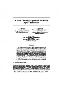
αi is the “degrees of freedom” and λi is a scale parameter. With λi = 1 and αi = 1, the Student t distribution is equal to the standard Cauchy distribution, and it tends to the standard Gaussian distribution as αi goes to infinity. √ αi Fig. 1 plots Student t densities for several values of αi , with equal mode, i.e setting λi = Γ( α+1 2 )/ αi π Γ( 2 ) for each density. Fig. 1 shows that for small αi , the Student t density gathers most of its probability mass around zero and exhibits “fatter tails” than the normal distribution. The Student t distribution is thus a relevant model for sparsity. Note that the i.i.d assumption of each sequence s˜i is only a working assumption 2 . Indeed, this assumption does not mean that our method is bound to fail when the coefficients sequences are not i.i.d (which is likely to happen for instance with MDCT coefficients of audio signals, because of the existence of time and frequency structures). 2 This

DRAFT

expression is used in several papers of Pham, see e.g [4]

January 21, 2005


5

Student t densities for α = [0.01 0.1 1 10] with equal mode

1

0.8

0.6

0.4 α 0.2

0 −5

Fig. 1.

−4

−3

−2

−1

0

1

2

3

4

5

Student t densities for α = [0.01, 0.1, 1, 10] with equal mode - The dash-lined plot is the Gaussian density with variance 1/2 π.

It only means that we choose not to use the inner correlation of the sequences, though this information could be used to design future separation schemes (see discussion in Section VI). The Student t distribution can be expressed as a Scale Mixture of Gaussians (SMoG) [24], such that Z +∞ 2 αi p(˜ si,k |αi , λi ) = dvi,k N (˜ si,k |0, vi,k ) IG vi,k | , 2 αi λ2i 0

(8)

where N (x|µ, v) and IG(x|γ, β) are the Gaussian and inverted-Gamma distributions, defined in Appendix I. Thus, introducing the auxiliary random variable vi,k , p(˜ si,k |αi , λi ) can be interpreted as a marginal density of the joint distribution p(˜ si,k , vi,k |αi , λi ), defined by p(˜ si,k , vi,k |αi , λi ) = p(˜ si,k |vi,k ) p(vi,k |αi , λi )

(9)

with

αi 2 p(˜ si,k |vi,k ) = N (˜ si,k |0, vi,k ) and p(vi,k |αi , λi ) = IG vi,k | , 2 αi λ2i

(10)

The fact that s˜i,k is Gaussian conditionally upon the variance vi,k of the Gaussian distribution in Eq. (8) is a very convenient property. Furthermore, the distribution of the variances vi,k is inverted-Gamma, which corresponds to the conjugate prior of vi,k in the expression of N (si,k |0, vi,k ), which means that the variance vi,k conditionally upon si,k , αi and λi will also be inverted-Gamma and thus easy to sample from (see Section IV-D). The Student t can thus be interpreted as an infinite sum of Gaussians, which contrasts with the finite sums of Gaussians used in [6], [11]. The Laplacian prior used in [7], [9] can also be expressed as a SMoG, with an exponential density on the variance vi,k [24]. Unfortunately this density does not lead to a distribution of vi,k conditionally upon s˜i,k (and the scale parameter) straightforward to sample from. In comparison with the Laplacian prior, the Student t prior has the advantage to offer a supplementary hyperparameter αi which controls the “peakness” of the distribution. January 21, 2005

DRAFT

6


In the following, we denote vk = [v1,k , . . . , vn,k ]T , v = [v0 , . . . , vN −1 ], α = [α1 , . . . , αn ] and λ = [λ1 , . . . , λn ]. 3) Mutual independence: We assume that the coefficients sequences of the sources are mutually independent, Qn such that p(˜s) = i=1 p(˜ si ). As pointed out in [10], the assumption of mutual independence of the coefficients of the sources on the basis can be considered more realistic than the mutual independence of the sources themselves, which is the standard assumption of ICA methods. ˜ is a i.i.d Gaussian noise with covariance σ 2 Im , and with σ unknown. 4) Noise properties: We assume that n We point out that when an orthonormal basis is used (i.e, Φ−1 = ΦT ), n is equivalently a Gaussian i.i.d noise with covariance σ 2 Im . We now present a MCMC approach to estimate the set of parameter of interest {˜s, A, σ} together with v and the hyperparameters {α, λ}. We define θ = {˜s, A, σ, v, α, λ}, and θ −y will denote the set of parameters in θ except y. For instance, θ −A = {˜s, σ, v, α, λ}. III. P RESENTATION OF THE G IBBS SAMPLER We derive in the following a Gibbs sampler to generate samples from the posterior distribution p(θ|˜ x). The obtained samples {θ (1) , . . . , θ (K) } then allows for computation a various point estimates, a standard one being the Minimum Mean Square Error (MMSE) estimate defined by Z ˆ M M SE = θ p(θ|˜ θ x) dθ

(11)

and which can be approximated by K X ˆ M M SE ≈ 1 θ θ (l) K

(12)

l=1

The Gibbs sampler only requires to be able to sample from the posterior distribution of certain subsets of parameters ˜ and the remaining parameters [25], [26]. Let {θ 1 , . . . , θ M } denote a partition of θ. The conditional upon data x Gibbs sampler works as follows: (0)

(0)

Initialize θ (0) = {θ 1 , . . . , θ M } for k = 1 : K + KBurnin do (k)

(k−1)

, . . . , θM

˜) ,x

(k)

(k)

(k−1)

(k−1)

θ 1 ∼ p(θ 1 |θ 2

(k−1)

θ 2 ∼ p(θ 2 |θ 1 , θ 3 (k) θ3

∼

.. .

(k)

, . . . , θM

(k−1) (k) (k) p(θ 3 |θ 1 , θ 2 , θ 4

(k)

(k)

˜) ,x

(k−1) ˜) . . . , θM , x

(k)

˜) θ M ∼ p(θ M |θ 1 , θ 2 , . . . , θ M −1 , x end for KBurnin represents the number of iterations required before the Markov chain {θ (1) , θ (2) , . . .} reaches its stationary distribution p(θ|˜ x). Thereafter, all samples are drawn from the desired stationary distribution. MCMC methods have the advantage to generate samples from the whole support of p(θ|˜ x), and thus to give an overall panorama of the posterior distribution of the parameters. When looking for a point estimate of θ, the MCMC DRAFT

January 21, 2005


7

approach prevents from falling into local modes of the posterior distribution, which is a common drawback of standard optimisation methods, like Expectation Maximisation or gradient type methods, which target at point estimates (such as Maximum A Posteriori estimates) from start. To implement the Gibbs sampler for θ = {˜s, A, σ, v, α, λ} we now need to derive the various densities of each parameter conditional upon the others and the data.

IV. C ONDITIONAL DENSITIES A. General outline ˜ ) of each parameter conditional upon the other parameters and the data The conditional distribution p(θ k |θ −k , x is written ˜) = p(θ k |θ −k , x

p(θ|˜ x) p(θ −k |˜ x)

(13)

Bayes’ theorem gives [27] p(θ|˜ x) =

p(˜ x|θ) p(θ) p(˜ x)

(14)

and it follows ˜) p(θ k |θ −k , x

=

p(˜ x|θ) p(θ) p(θ −k |˜ x) p(˜ x)

∝ p(˜ x|θ) p(θ)

(15) (16)

Thus, the required conditional distributions are proportional to the likelihood of the data times the priors on the parameters. 1) Prior structure: Assuming independence of the mixing matrix, the noise variance and the sources parameters, we have: p(θ)

= p(˜s, A, σ, v, α, λ)

(17)

= p(˜s|v) p(v|α, λ) p(α) p(λ) p(A) p(σ)

(18)

2) Likelihood: Under Gaussian noise and sources coefficients i.i.d assumptions, the likelihood is written p(˜ x|θ)

= p(˜ x|A, ˜s, σ) =

N −1 Y

(19)

N (˜ xk |A ˜sk , σ 2 Im )

(20)

k=0

=

1 (2 π σ 2 )

Nm 2

N −1 1 X exp(− 2 k˜ xk − A ˜sk k2F ) 2σ

(21)

k=0

where N (x|µ, Σ) denotes the multivariate Gaussian distribution defined in Appendix I. Using the priors structure and the expression of the likelihood we now give resulting conditional densities of each parameter upon the others and the data. In the following sections we give results without derivations; some details are given in appendices. January 21, 2005

DRAFT

8


B. Sampling ˜s We show in Appendix II-A ˜) = p(˜s|θ −˜s , x

N −1 Y

N (˜sk |µ˜sk , Σ˜sk )

(22)

k=0

where Σ˜sk =

1 σ2

−1

AT A + diag (vk )

−1

and µ˜sk =

1 σ2

˜ k (and where diag (u) is the diagonal matrix Σ˜sk AT x

whose main diagonal is given by u). Notice that ˜sk being Gaussian conditionally upon vk , the latter expressions are nothing but the formula of linear estimation of a Gaussian vector parameter in Gaussian noise [27]. C. Sampling A and σ ˜ ) and p(σ|θ −σ , x ˜ ), as It is possible to sample A and σ separately, by evaluating and sampling from p(A|θ −A , x ˜ ), which is a better strategy as it is done in [17]. But it is also possible to sample directly from p(A, σ|θ −(A,σ) , x recommended to sample as many parameters as possible together to accelerate convergence of the Gibbs sampler ˜ ) is equivalent to sampling σ (k) from p(σ|θ −(A,σ) , x ˜ ) and [25], [26]. Sampling (A(k) , σ (k) ) from p(A, σ|θ −(A,σ) , x ˜ ) [26]. then sample A(k) from p(A|θ −(A,σ) , σ (k) , x It is shown in Appendix II-C that with Jeffrey’s uninformative prior [28] p(σ) = 1/σ we have ˜ ) ∼ IG(ασ , βσ ) (σ 2 |θ −(A,σ) , x

(23)

with ασ =

(N − n) m 2

and βσ = P m PN −1 i=1

˜2i,k k=0 x

−

P

N −1 k=0

x ˜i,k ˜sTk

2 P N −1 k=0

˜sk ˜sTk

−1 P

N −1 k=0

x ˜i,k ˜sk

(24)

˜ ). Let r1 , . . . , rm be the n × 1 vectors denoting the transposed rows Now we need to sample from p(A|θ −A , x of A, such that AT = [r1 . . . rm ]. We show in Appendix II-B that with (Jeffrey’s) uninformative uniform prior p(A) ∝ 1 we have ˜) = p(A|θ −A , x

m Y

N (ri |µri , Σr )

(25)

i=1

PN −1 with Σr = σ 2 ( k=0 ˜sk ˜sTk )−1 and µri =

1 σ2

Σr

PN −1 k=0

x ˜i,k ˜sk .

Because of the inherent source separation indetermination on gain, a scale factor has to be fixed, whether on the mixing matrix, or on the sources. We discuss several possibilities: •

indetermination fixed in A: one option is to set a row ri0 to fixed values, for instance ones. We then sample from the other rows and the scale parameters λi . This has the advantage to initialize easily A when a rough estimate of the mixing matrix is available (for instance provided by a clustering method in the space of the observations [10], [29]): only divide the columns of A by the values of the chosen row ri0 , and initialize the Gibbs sampler with the resulting matrix. However, this can be problematic if one source has a low contribution in the corresponding sensor i0 . Another option is to set the norms of the columns of A to a fixed value, but this imply to sample the columns of A on a sphere, which is not straightforward.

DRAFT

January 21, 2005


•

9

indetermination fixed on the sources: we can set the scale parameters λi to fixed values and then sample from all the rows of the mixing matrix. However we found out in practice that the initialization of A is difficult. Initializing the mixing matrix with a matrix of zeros does not give satisfactory results because a column of A gets stuck to nearly zero values, and initializing A with entries in a correct range of values is not straightforward. The ideal situation is when a rough estimate of A is available. In that case, the scale parameters of the Student t distributions can be estimated with a standard method [30] (by setting the degrees of freedom to a reasonable fixed value or possibly estimating them) providing values which can be used as initializations of λi in the Gibbs sampler. Then we can proceed by sampling from all the rows of A in order to refine the mixing matrix estimate.

To obtain the results presented in Section V we chose for its simplicity the option consisting in setting the first row of A to ones and sampling from the other rows and the scale parameters of the sources. However we acknowledge that the other schemes are to be investigated.

D. Sampling v Since the likelihood does not depend on the parameters {v, α, λ}, their posterior distributions are conditionally ˜ . The variances vi,k having an inverted-Gamma (conjugate) prior we obtain easily (Appendix II-D): independent of x ˜) = p(v|θ −v , x

N −1 Y n Y

IG vi,k |γvi , βvi,k

(26)

k=0 i=1

with γvi = (αi + 1)/2 and βvi,k = 2/(˜ s2i,k + αi λ2i ).

E. Sampling α We have (Appendix II-E) ˜) ∝ p(α|θ −α , x

−( n Y P i=1

with Ri =

PN −1

1 k=0 vi,k

and Pi =

αi 2

+1)

i

QN −1 k=0

Γ( α2i )N

αi λ2i 2

αi2N

αi λ2i exp − Ri p(αi ) 2

(27)

vi,k . We choose an uninformative uniform prior on αi and set p(α) ∝ 1.

˜ ) is not straightforward to sample from and since the precise value αi for each As the distribution of (α|θ −α , x source is unlikely to be important, in practice we sample α from a uniform grid of discrete values with probability masses given by Eq. (27).

F. Sampling λ Finally, with the uninformative Jeffreys prior p(λi ) = 1/λi , we have (Appendix II-E): ˜ ) ∼ G (γλi , βλi ) (λ2i |θ −λ , x

(28)

with γλi = (αi N )/2 and βλi = 2/(αi Ri ), and where G(γ, β) is the Gamma distribution given in Appendix I. January 21, 2005

DRAFT

10


Initialize θ (0) = {˜ s(0) , A(0) , σ (0) , v(0) , α(0) , λ(0) } for k = 1 : K + KBurnin do ˜ ˜) s(k) ∼ p(˜ s|A(k−1) , σ (k−1) , v(k−1) , x ˜) σ (k) ∼ p(σ|˜ s(k) , x ˜) A(k) ∼ p(A|˜ s(k) , σ (k) , x v(k) ∼ p(v|˜ s(k) , α(k−1) , λ(k−1) ) α(k) ∼ p(α|v(k) , λ(k−1) ) λ(k) ∼ p(λ|v(k) , α(k) ) end for

TABLE I G IBBS SAMPLER FOR SOURCE SEPARATION

OF

S TUDENT t SOURCES .

G. Summary At this point all the posterior conditional distributions required for the Gibbs sampler have been presented. All we have to do now is decompose the observations x into the given basis Φ, and apply the Gibbs sampler described ˜ . The several steps of the sampler are recapitulated in Table I and in Section III to the sequences of coefficients x emphasizes the dependencies between the several parameters. Samples from ˜s and A are thus obtained, and MMSE estimates are computed using Eq. (12). Estimates of the original sources s can be obtained by applying Φ−1 to the estimate of ˜s. We stress that thanks to the Student t model, expressed as a SMoG with inverted-Gamma distributed variances, all the posterior conditional distributions are easy to sample from. In the following section we consider the separation of audio signals decomposed on a MDCT basis, a local cosine lapped transform [14] which has proven to give good sparse approximations of audio signals, with many coding applications ([31], [32]). We first consider a noisy underdetermined mixing in Section V-A and then a noisy determined mixing in Section V-B. Robustness of the methods over several mixing matrices are investigated in Section V-C. The results are then discussed in Section V-D.

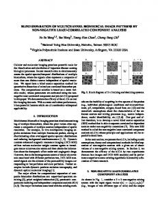
V. R ESULTS A. Underdetermined mixture We first study a mixture of n = 3 audio sources (speech, piano, guitar) with m = 2 observations. The mixing matrix is given in Table II. We set σ = 0.03, which corresponds to approximatively 20dB noise on each observation. The signals are sampled at 8kHz with length N = 65356 ( ≈ 8s). We used a MDCT basis to decompose the observations, with sine window of length 64ms (512 samples). Windows of lengths 32ms and 128ms were also tried but led to slightly poorer results. Fig. 2 shows scatter plots of the observations in the time domain and the transform domain. Fig. 2 (b) shows the sparsification induced by the MDCT decomposition: the directions of the mixing matrix columns clearly appear, contrary to Fig. 2 (a). DRAFT

January 21, 2005


Fig. 2.

11

(a) Scatter plot of x1 w.r.t x2 . (b) Scatter plot of x ˜1 w.r.t x ˜2 - the dashed lines represent the directions of the mixing matrix.

We ran 5000 iterations of the Gibbs sampler, and MMSE estimates of A and ˜s where computed from the final 1000 samples. The different parameters were initialised with the following values (using MATLAB notation):

˜s ones(n × N )

r2 h

0

0

i 0

σ

v

α

λ

0.1

ones(n × N )

ones(1, n)

0.1∗ones(1, n)

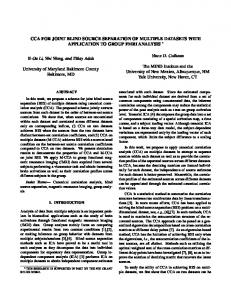
The discrete values from which the degrees of freedom αi are sampled from are chosen linearly spaced between 0.05 and 5, with step size 0.05. We compared our method (referred to as “t + MCMC”) with the one in [11], which uses a mixture of two Gaussians to model the source coefficients distribution: one state ‘on’ corresponding to a high variance Gaussian, one state ‘off’ corresponding to a small variance Gaussian (in fact, the method intrinsically sets the ’off’ state variance to zero to solve identifiabilty problems inherent to the model, see [11]). The method, referred to as “FMoG + EM”, estimates the mixing matrix, the noise covariance and the weights in the mixtures of Gaussians with a EM-based procedure. MMSE estimates of the sources are then inferred from the estimated parameters and the data. The method was run for 50 iterations, and convergence was observed after 30 iterations. Fig. 4 plots samples drawn from the second row r2 of A, α, λ and σ throughout the iterations of the Gibbs sampler. Table II shows the mixing matrices estimated by the two methods, together with the standard variations in the case of the t + MCMC method (the FMoG + EM method only provides point estimates). Fig. 3 plots the distributions of the coefficients of the original sources compared to the estimated Student t densities of each source. Table III provides separation quality criteria for the sources estimates given by the two methods. The criteria used are described in [33]. Basically, the SDR (Source to Distortion Ratio) provides an overall separation performance criterion, the SIR (Source to Interferences Ratio) measures the level of interferences from the other sources in each source estimate, SNR (Source to Noise Ratio) measures the error due to the additive noise on the sensors January 21, 2005

DRAFT

12


Source 1

Source 2

0

10 p(s)

−2

10

−2

−2

10

−4

10

10

−4

−5

Fig. 3.

0

0

10 p(s)

p(s)

10

Source 3

0 s

5

10

−5

0 s

5

−4

−2

0 s

2

4

Distributions of the sequences s˜i (full lines) compared to the estimated Student t densities (dot lines) - notice the Y-axis log-scale.

Original matrix 3 2 1 1 1 5 4 A= 0.8 1.3 − 0.9

t + MCMC 2

1 6 ˆ = 6 0.7827 A 4 (±0.0026)

FMoG + EM

1

1

3

7 − 0.9021 7 5 (±0.0028)

1.2950 (±0.0018)

2 ˆ =4 A

3

1

1

1

0.7545

1.3249

− 0.9001

5

TABLE II

E STIMATES OF A FOR THE UNDERDETERMINED MIXTURE .

and the SAR (Source to Artifacts Ratio) measures the level of artifacts in the source estimates. We point out that the performance criteria are invariant to a change of basis, so that figures can be computed either on the time sequences (ˆs compared to s) or the MDCT coefficients (ˆ˜s compared to ˜s). The estimated sources can be listened to at http://www-sigproc.eng.cam.ac.uk/˜cf269/ieee_sap05/sound_files.html, which is perhaps the best way to assess the audio quality of the results.

sˆ1

sˆ2

sˆ3

SDR

SIR

SAR

SNR

SDR

SIR

SAR

SNR

SDR

SIR

SAR

SNR

t + MCMC

3.2

13.8

3.9

20.3

8.1

15.1

9.2

26.9

16.5

25.7

18.9

21.8

FMoG + EM

2.4

16.2

2.7

34.5

5.9

20.7

6.0

40.7

6.3

44.7

6.3

39.5

TABLE III

P ERFORMANCE CRITERIA FOR THE UNDERDETERMINED MIXTURE .

DRAFT

January 21, 2005


(a) r2

1.5

(b) λ

0.2

1

13

0.15

0.5 0.1 0 0.05

−0.5 −1

0

1000

2000

4000

5000

(c) α

5

0

0.2

3

0.15

2

0.1

1

0.05

0

1000

2000

3000

0

1000

4000

5000

0

2000

3000

4000

5000

4000

5000

(d) σ

0.25

4

0

Fig. 4.

3000

0

1000

2000

3000

Samples from the different parameters obtained with the Gibbs sampler for the underdetermined mixture.

B. Determined mixture We now give results on a determined mixture (m = n). The same sources are used, with mixing matrix given in Table IV. We set σ = 0.1, which approximatively corresponds to 9.5 dB noise on each observation. As before MDCT decompositions were performed with 64ms window length and 5000 iterations of the Gibbs sampler were run (with same initialisations), MMSE estimates being computed from the last 1000 iterations. The FMoG + EM method was used with 30 iterations, and convergence was observed after 20 iterations. For comparison, we also show the results provided by the standard ICA algorithm JADE [34], which estimates a separating matrix via jointdiagonalization of a set of cumulant matrices, and apply the obtained matrix to the observations, without denoising of the sources estimates. Fig. 5 plots samples drawn from r2 , r3 , α, λ and σ throughout the iterations of the Gibbs sampler. Table IV shows the estimated mixing matrices, Table V shows quality criteria of the estimated sources.

C. Robustness to mixing matrix In this section we study the robustness of the two methods over several mixing matrices, in particular over matrices with “close” columns. We used the same audio sources as before, though we now consider only 1s excerpts of January 21, 2005

DRAFT

14


(a) r2

1.5 1

1

0.5

0.5

0

0

−0.5

−0.5

−1

0

1000

2000

3000

(c) λ

0.08

4000

−1

5000

0

1000

2000

(d) α

2.5

0.06

(b) r3

1.5

3000

4000

5000

(e) σ

2

0.25

1.5

0.2

1

0.15

0.5

0.1

0.04 0.02 0

Fig. 5.

0

2000

4000

0

0

2000

0.05

4000

0

2000

4000

Samples from the different parameters obtained with the Gibbs sampler for the overdetermined mixture.

them. We designed 4 mixing matrices of the following form:  1 1 A= tan ψ1 tan ψ2

1 tan ψ3

 (29)



We considered the 4 sets of values of {ψ1 , ψ2 , ψ3 } indicated in Table VI. For visibility we plot the independent component directions generated by the several matrices in Fig. 6. The first case corresponds to widely spread directions, the second and third cases correspond to two closely spread directions and the fourth case correspond to three closely spread directions. The initialisation of the parameters in the Gibbs sampler was chosen as before; the mixing matrix in the FMoG + EM method was initialized with a matrix of the form of Eq. (29) with nearly zero angles (the method does not accept strictly zero angles), however random initialisations lead to similar results. Noise with power σ = 0.03 was added on the observations, providing input SNRs in the range 20-30 dB. The estimates of {ψ1 , ψ2 , ψ3 } provided by both methods are given in Table VI. Corresponding separation quality criteria are given in Table VII D. Discussion 1) Separation quality assessment: A major advantage of the Student t model over the FMoG model is sound quality. These can be perceived by listening to the sound samples, but also by looking at the SARs of the source DRAFT

January 21, 2005


15

Original matrix 2

1

1

6 A=6 40.8

7 − 0.97 5

1.3 − 0.7

1.2

3

1 1.1

t + MCMC 2

1

1

6 6 0.7938 6 6 ˆ A=6 6 ± (0.0046) 6 6 1.1954 4 ± (0.0058)

3

1

7 − 0.8978 7 7 7 (±0.0049) 7 7 7 1.0996 7 5 ± (0.0042)

1.3038 (±0.0050) − 0.7039 ± (0.0046)

FMoG + EM 2

1

1

6 ˆ = 60.7790 A 4 1.1864

1

1.3181

3

7 − 0.88727 5

− 0.7182

1.1069

JADE 2

1

1

6 ˆ = 60.7814 A 4 1.3449

1

1.3226

3

7 − 0.89747 5

− 0.7920

0.8710

TABLE IV

E STIMATES OF A FOR THE OVERDETERMINED MIXTURE .

sˆ1

sˆ2

sˆ3

SDR

SIR

SAR

SNR

SDR

SIR

SAR

SNR

SDR

SIR

SAR

SNR

t + MCMC

12.3

35.7

13.9

17.5

15.4

36.8

17.0

20.6

13.4

35.0

15.2

18.3

FMoG + EM

5.6

36.7

5.6

33.5

6.5

48.4

6.5

35.0

5.9

37.0

5.9

31.0

JADE

8.1

18.8

-

8.5

5.3

15.6

-

5.8

5.7

37.3

-

5.7

TABLE V

P ERFORMANCE CRITERIA FOR THE OVERDETERMINED MIXTURE .

estimates which are higher using the t model in all the presented simulations. The t model provides estimates which sound much more natural that the FMoG model. Fig. 3 show the very good fit between the estimated Student t distributions and the histograms of the MDCT coefficients of the sources. The main advantage of the FMoG model is noise reduction as measured with SNR. SNRs of the sources estimates are better with the FMoG model than with the t model. We think this is because the model sets the ’off’ state variance to zero and thus performs a thresholding of the MDCT coefficients, which might eliminate small coefficients originated from the additive noise on the observations. The t model gives slightly poorer interference rejection in the underdetermined case and similar performances to the FMoG model in the determined case (and no interference can be heard over 30dB SIR). When considering January 21, 2005

DRAFT

16


Case 1

Case 2 ψ3

ψ3

−0.5 −1

Fig. 6.

ψ1 0

0.5 x1

Case 4 ψ3

ψ3

ψ2 0.5

0.5

0

0

0

−0.5 −1

ψ2

−0.5

ψ1 0

x2

0.5

x2

ψ2

0

x2

x2

0.5

Case 3

−1

0.5 x1

ψ1 0

0.5 x1

ψ2 ψ1

−0.5 −1

0

0.5 x1

Directions generated by the several matrices in the 4 cases studied

Case 1 ψ1

ψ2

ψ3

True value (deg)

-45

15

75

t + MCMC

-44.6

16.4

75.3

FMoG + EM

-46.3

17.5

75.6

Case 2 ψ1

ψ2

ψ3

True value (deg)

-45

66

75

t + MCMC

-43.9

66.2

75.4

FMoG + EM

-49.3

86.5

71.9

ψ3

Case 3 ψ1

ψ2

True value (deg)

-45

-36

75

t + MCMC

-45.8

-35.6

75.2

FMoG + EM

-40.6

-83.6

75.2

ψ2

ψ3

Case 4 ψ1 True value (deg)

57

66

75

t + MCMC

56.9

66.2

75.0

FMoG + EM

57.6

66.2

74.7

TABLE VI E STIMATED ANGLES

DRAFT

January 21, 2005


17

Case 1 sˆ1

sˆ2

sˆ3

SDR

SIR

SAR

SNR

SDR

SIR

SAR

SNR

SDR

SIR

SAR

SNR

t + MCMC

9.3

19.1

10.3

20.5

5.9

14.5

6.8

23.5

14.3

22.5

15.3

26.5

FMoG + EM

5.2

22.3

5.4

38.5

4.41

16.3

4.8

32.6

5.9

28.0

6.0

42.0

SAR

SNR

SDR

SIR

SAR

SNR

Case 2 sˆ1

sˆ2 SDR

SIR

sˆ3

SDR

SIR

SAR

SNR

t + MCMC

13.8

21.7

16.1

20.1

3.6

10.9

4.9

27.3

3.3

11.5

4.4

28.6

FMoG + EM

5.4

30.9

5.4

36.2

-30.9

-22.7

-7.5

40.7

-0.4

3.5

3.5

47.1

SAR

SNR

SDR

SIR

SAR

SNR

Case 3 sˆ1 SDR

SIR

t + MCMC

5.2

FMoG + EM

-0.4

sˆ2 SDR

SIR

sˆ3

SAR

SNR

14.6

5.9

24.1

4.1

9.7

6.1

21.9

22.1

33.6

25.3

25.5

0.3

10.2

36.0

-27.0

-15.7

-10.8

29.1

4.6

32.3

4.6

40.0

Case 4 sˆ1

sˆ2

sˆ3

SDR

SIR

SAR

SNR

SDR

SIR

SAR

SNR

SDR

SIR

SAR

SNR

t + MCMC

8.8

20.0

9.4

21.6

5.7

13.7

6.6

31.0

11.1

23.6

11.6

24.7

FMoG + EM

4.4

23.1

4.5

32.5

4.7

15.8

5.2

36.2

7.5

34.6

7.5

30.5

TABLE VII

P ERFORMANCE CRITERIA FOR THE DIFFERENT CASES .

an overdetermined mixture with m = 4 sensors (with rT4 = [−0.6 1.5 0.9]), the SIR of each source estimates rise to respectively 48.9, 50.0 and 46.2 dB with the t + MCMC method and to 44.1, 44.7 and 39.1 dB with the FMoG + EM method. However the SARs obtained by both methods do not increase, which show the limitations of the priors studied. Notice the benefit of using sparsity for denoising purpose: the SNRs obtained by the methods t + MCMC and FMoG + EM are much higher than those obtained with JADE. The mixing matrices are well estimated by both methods in both cases, with slightly better performance with the t + MCMC method. One advantage of the MCMC approach over EM is that standard variations of the estimated parameters can be computed easily. The difference of convergence speed of the mixing matrix parameters between the underdetermined and determined cases is striking when looking at Fig. 4 a) and Fig. 5 a) & b); in the determined case, a good estimate of the mixing matrix can be obtained within 100 iterations. The faster convergence and better results are explained by the fact that in the determined context µ˜sk is simply the result of the application of the ˜k. (weighted) pseudo-inverse of A to x Another reason for the faster convergence in the determined case is the higher level of noise. The higher the level of input noise the less peaky the likelihood becomes, thus the conditional posterior distributions of the parameters have a wider support and the Gibbs sampler “mixes” better [26]. When applying the Gibbs sampler to January 21, 2005

DRAFT

18


the underdetermined mixture presented in V-A with a lower noise level (σ = 0.01 instead of σ = 0.03), the estimate of r2 is slightly more accurate (with standard deviations divided by two) and the SNRs of the sources estimates decrease by 7dB, but convergence is only obtained after approximatively 4000 iterations (instead of approximatively 1500 when σ = 0.03). 2) Separation performance with respect to mixing matrix: Results of Section V-C emphasize another advantage of the MCMC approach compared with EM: robustness to mixing matrix. The t + MCMC method converges to the correct angle values in all 4 cases. On the contrary, the FMoG + EM approach only converges to the correct angles in case 1 and case 4. The problem encountered with the latter method is as follows: the clusters generated by the two close column directions in case 2 and case 3 are regarded as a single cluster: ψˆ3 is fitted between ψ2 and ψ3 in case 2, ψˆ1 is fitted between ψ1 and ψ2 in case 3. In these cases the isolated direction is well estimated (ψ1 in case 2 and ψ3 in case 3) and the remaining direction of the estimated matrix is completely wrong. However the FMoG + EM method performs well in case 4 when all the columns of A are closely spread. It seems to be meaning that the problem encountered in case 2 and 3 is not only a problem of convergence of the algorithm to local modes, but also a matter of how the method “interprets” the data (similar results were obtained over several random initialisations of the EM algorithm). As already mentioned in Section III, the better robustness of the MCMC approach derives from the fact that the algorithm explores all the space of possible values of p(θ|˜ x) whereas the EM approach only updates point estimates. Interestingly, Table VII show that separation quality in case 1 is only slightly better than in case 4. In cases 2 and 3, the source along the isolated direction is very well estimated, much better that the 2 other sources, which SDRs surprisingly do not meet the values obtained in case 4. 3) Computational issues: The MCMC approach has significantly higher computational burden than the EM approach, in particular the one designed in [11] which falls in the category of Alternating Expectation Conditional Maximization methods, and thus shows faster convergence than the standard EM algorithm. In Matlab, 1000 iterations of the t + MCMC method applied to a mixtures of n = 3 sources with N = 65536 require approximatively 3 hours on a Mac G4 cadenced at 1.25GHz while it takes only a few minutes for the FMoG + EM method to converge. Fig. 4 shows that in the underdetermined case several hundreds of iterations are required before convergence. However, Fig. 5 shows that in the determined case convergence is obtained within only 100 iterations, which, taking into account the increased robustness and audio quality, challenges the EM based method. In the underdetermined case convergence can be very much accelerated by initialising the mixing parameters with a rough estimate of A, obtained with a clustering method like in [10], [29] or simply using the FMoG + EM method. Depending on the quality of the initialization, good estimates of the sources can be obtained within 1000 iterations. VI. C ONCLUSION We have presented a Bayesian approach to perform separation of linear instantaneous mixtures of sources having a sparse representation on a basis. We used a Student t distribution to model the sparsity of the coefficients. This distribution has the advantage that it can be expressed as a SMoG with an inverted-Gamma mixing weight DRAFT

January 21, 2005


19

function. This property allowed us to calculate easily the conditional posterior distributions required to design a Gibbs sampler. MMSE estimates of the mixing matrix and the sources were computed, and compared with an EM approach using a FMoG model with two states. The primary aim of this article is show the good properties of the Student t prior for modelling sparsity. The MCMC approach is very robust but also computationally demanding. Possible ways to alleviate this would be EM approaches based on the Student t prior, in order to keep the increased audio quality with respect to the FMoG prior, while alleviating the computational burden implied the MCMC approach. However, this is likely to be at the expense of robustness to initialization and mixing matrix. Other perspectives are to extend our method to the case of overcomplete dictionaries, which would improve sparsity of the coefficients of the representation of the sources in the dictionary, and is thus likely to improve separation. As a first step an easy extension is the use of overcomplete lapped cosine transforms. Another option is the use of Gabor representations. Following the approach in [15] we can also consider using an indicator variable framework (i.e, a prior model of the form p(˜ si,k |αi , λi ) = γi,k δ0 (˜ si,k )+(1−γi,k ) t(˜ si,k |αi , λi ), with γi,k ∈ {0, 1}). Besides further enforcing sparsity of the coefficients, this framework would easily allow to model audio signals time-frequency structures by choosing proper priors on γ to model harmonic structures. Another useful direction will be making comparisons between the use of Student t prior and Exponential Power Distributions family (to which the Laplacian belongs), which can also be expressed as SMoG [35], though the weight function does not lead to straightforward conditional distributions, but sampling could be achieved by rejection sampling schemes [26].

ACKNOWLEDGEMENT Many thanks to Laurent Daudet for providing us with the MDCT code.

A PPENDIX I S TANDARD DISTRIBUTIONS Multivariate Gaussian

1

N (x|µ, Σ) = |2π Σ|− 2 exp − 12 (x − µ)T Σ−1 (x − µ) G(x|γ, β) =

Gamma

IG(x|γ, β) =

inverted-Gamma

xγ−1 Γ(γ) β γ −(γ+1)

x Γ(γ) β γ

exp(− βx ) I[0,+∞) (x)

exp(− β1x ) I[0,+∞) (x)

The inverted-Gamma distribution is the distribution of 1/X when X is Gamma distributed.

A PPENDIX II D ERIVATIONS OF CONDITIONAL DISTRIBUTIONS ˜) A. Expression of p(˜s|θ −˜s , x We have: ˜ ) ∝ p(˜ p(˜s|θ −˜s , x x|A, ˜s, σ) p(˜s|v) January 21, 2005

(30) DRAFT

20


With p(˜s|v) =

QN −1 k=0

QN −1

p(˜sk |vk ) =

k=0

N (˜sk |0, diag (vk )) and with Eq. (20), we have

˜) ∝ p(˜s|θ −˜s , x

N −1 Y

N (˜ xk |A ˜sk , σ 2 Im ) N (˜sk |0, diag (vk ))

(31)

k=0

The product of Gaussians for each k can be easily rearranged as another Gaussian function of ˜sk , leading to Eq. (22).

˜) B. Expression of p(A|θ −A , x ˜ k and a denote the m × n m matrix and the n m × 1 vector defined by Let S     ˜sTk r1 0     .     . ˜k =  .. S  and a =  ..      ˜sTk rm 0

(32)

By construction, we have: ˜k a A ˜sk = S

(33)

Of course the estimation of a is equivalent to the estimation of A, and we have: ˜ ) ∝ p(˜ p(a|θ −a , x x|a, ˜s, σ) p(a)

(34)

Without further information on the mixing matrix, we assume uninformative uniform prior on A and set p(a) ∝ 1. Q −1 ˜ k a, σ 2 Im ), which can be rearranged as the ˜) ∝ N With Eq. (20) and (33), we have then p(a|θ −a , x xk |S k=0 N (˜ exponential of a quadratic form in a, such that ˜ ) = N (a|µa , Σa ) p(a|θ −a , x with Σa = σ 2

P

N −1 k=0

˜T S ˜ S k k

−1

and µa =

1 σ2

Σa

(35)

PN −1 ˜ T ˜ k . It appears that Σa is block-diagonal, and the k=0 Sk x

rows of A are thus independent, leading, after simplifications, to Eq. (25).

˜) C. Expression of p(σ|θ −(A,σ) , x We have: ˜ ) ∝ p(˜ p(σ|θ −(A,σ) , x x|θ −A ) p(σ)

(36)

and Z p(˜ x|θ −A )

=

p(˜ x, A|θ −A )dA

(37)

p(˜ x|θ) p(A)dA

(38)

ZA = A

Assuming uniform prior p(A) ∝ 1, the evaluation of p(˜ x|θ −A ) thus requires integrating the likelihood over A, or, in vector form, over a. The likelihood can be written p(˜ x|θ) =

DRAFT

1 (2 π σ 2 )

Nm 2

exp −

1 −1 T (a − µa )T Σ−1 a (a − µa ) + c − µa Σa µa 2

(39)

January 21, 2005


with c =

1 σ2

PN −1 k=0

21

˜ Tk x ˜ k and with Σa and µa defined before. The exponential quadratic form in a integrating to x

1

|2 π Σa | 2 , it follows

1

p(˜ x|θ −A ) =

|2 π Σa | 2 (2 π σ 2 )

Nm 2

exp −

1 c − µTa Σ−1 a µa 2

Expanding µTa Σ−1 a µa , grouping the terms in σ we obtain, with Eq. (36) (N −n) m 1 1 ˜) ∝ exp − p(σ). p(σ|θ −(A,σ) , x σ βσ σ 2

(40)

(41)

With p(σ) = 1/σ, it is possible to show that σ has a square root inverted-Gamma distribution, (which is the 1

distribution of X − 2 when X is Gamma distributed), leading to Eq. (23). ˜) D. Expression of p(v|θ −v , x We have ˜ ) ∝ p(˜s|v) p(v|α, λ) p(v|θ −v , x

(42)

Owing to sources coefficients i.i.d and mutual independence assumptions we have p(˜s|v) p(v|α, λ) =

N −1 Y n Y

p(˜ si,k |vi,k ) p(vi,k |αi , λi )

(43)

k=0 i=1

The product p(˜ si,k |vi,k ) p(vi,k |αi , λi ) can be expressed straightforwardly (up to a constant) as an inverted-Gamma density function with parameters γvi and βvi,k defined in Section IV-D ˜ ) and p(λ|θ −λ , x ˜) E. Expressions of p(α|θ −α , x We have ˜ ) ∝ p(v|α, λ) p(α) p(α|θ −α , x

Q

(44)

˜ ) ∝ p(v|α, λ) p(λ) p(λ|θ −λ , x (45) N −1 k=0 p(vi,k |αi , λi ) p(αi ) we get directly Eq. (23). Similarly, with p(v|α, λ) p(λ) =

Qn With p(v|α, λ) p(α) = i=1 Qn QN −1 i=1 k=0 p(vi,k |αi , λi ) p(λi ), we get

˜) ∝ p(λ|θ −λ , x

n Y

αi Si 2 λi p(λi ) λiαi N exp − 2 i=1

(46)

With p(λi ) = 1/λi , it is possible to show that λi has a square root-Gamma density (which is the distribution of 1

X 2 when X is Gamma distributed), leading to Eq. (28). R EFERENCES [1] J.-F. Cardoso, “Blind signal separation: statistical principles,” Proceedings of the IEEE. Special issue on blind identification and estimation, vol. 9, no. 10, pp. 2009–2025, Oct. 1998. [2] A. Hyvärinen, J. Karhunen, and E. Oja, Independent Component Analysis.

New York, NY: John Wiley & Sons, 2001.

[3] A. Belouchrani, K. Abed-Meraim, J.-F. Cardoso, and E. Moulines, “A blind source separation technique based on second order statistics,” IEEE Trans. Signal Processing, vol. 45, no. 2, pp. 434–444, Feb. 1997.

January 21, 2005

DRAFT

22


[4] D.-T. Pham and J.-F. Cardoso, “Blind separation of instantaneous mixtures of non stationary sources,” IEEE Trans. Signal Processing, vol. 49, no. 9, pp. 1837–1848, Sep. 2001. [5] C. Févotte and C. Doncarli, “Two contributions to blind source separation using time-frequency distributions,” IEEE Signal Processing Letters, vol. 11, no. 3, Mar. 2004. [6] B. A. Olshausen and K. J. Millman, “Learning sparse codes with a mixture-of-Gaussians prior,” in Advances in Neural Information Processing Systems, S. A. Solla and T. K. Leen, Eds.

MIT press, 2000, pp. 841–847.

[7] M. S. Lewicki and T. J. Sejnowski, “Learning overcomplete representations,” Neural Computations, vol. 12, pp. 337–365, 2000. [8] M. Girolami, “A variational method for learning sparse and overcomplete representations,” Neural Computation, vol. 13, no. 11, pp. 2517–2532, 2001. [9] T.-W. Lee, M. S. Lewicki, M. Girolami, and T. J. Sejnowski, “Blind source separation of more sources than mixtures using overcomplete representations,” IEEE Signal Processing Letters, vol. 4, no. 4, Apr. 1999. [10] M. Zibulevsky, B. A. Pearlmutter, P. Bofill, and P. Kisilev, “Blind source separation by sparse decomposition,” in Independent Component Analysis: Principles and Practice, S. J. Roberts and R. M. Everson, Eds.

Cambridge University Press, 2001.

[11] M. Davies and N. Mitianoudis, “A simple mixture model for sparse overcomplete ICA,” IEE Proceedings on Vision, Image and Signal Processing, Feb. 2004. [12] R. Gribonval, “Sparse decomposition of stereo signals with matching pursuit and application to blind separation of more than two sources from a stereo mixture,” in Proc. ICASSP, Orlando, Florida, May 2002. [13] A. Jourjine, S. Rickard, and O. Yilmaz, “Blind separation of disjoint orthogonal signals: Demixing n sources from 2 mixtures,” in Proc. ICASSP, vol. 5, Istanbul, Turkey, Jun. 2000, pp. 2985–2988. [14] S. Mallat, A wavelet tour of signal processing.

Academic Press, 1998.

[15] P. J. Wolfe, S. J. Godsill, and W.-J. Ng, “Bayesian variable selection and regularisation for time-frequency surface estimation,” J. R. Statist. Soc. Series B, 2004. [16] D. Wipf, J. Palmer, and B. Rao, “Perspectives on sparse Bayesian learning,” in Advances in Neural Information Processing Systems 16, S. Thrun, L. Saul, and B. Schölkopf, Eds.

Cambridge, MA: MIT Press, 2004.

[17] C. Févotte, S. J. Godsill, and P. J. Wolfe, “Bayesian approach for blind separation of underdetermined mixtures of sparse sources,” in Proc. 5th International Conference on Independent Component Analysis and Blind Source Separation (ICA 2004), Granada, Spain, 2004, pp. 398–405. [18] K. H. Knuth, “A Bayesian approach to source separation,” in Proc. 1st International Workshop on Independent Component Analysis and Signal Separation, Aussois, France, Jan. 1999, pp. 283–288. [19] A. Mohammad-Djafari, “A Bayesian approach to source separation,” in Proc. 19th International Workshop on Bayesian Inference and Maximum Entropy Methods (MaxEnt99), Boise, USA, Aug. 1999. [20] D. B. Rowe, “A Bayesian approach to blind source separation,” Journal of Interdisciplinary Mathematics, vol. 5, no. 1, pp. 49–76, 2002. [21] P.-O. A. S. Sénécal, “Bayesian separation of discrete sources via Gibbs sampling,” in Proc. International Workshop on Independent Component Analysis and Blind Signal Separation, Helsinki, Finland, 2000, pp. 566–572. [22] C. Andrieu, A. Doucet, and S. J. Godsill, “Bayesian blind marginal separation of convolutively mixed discrete sources,” in Proc. IEEE Workshop on Neural Networks for Signal Processing, Cambridge, 1998. [23] C. Andrieu and S. J. Godsill, “Bayesian separation and recovery of convolutively mixed autoregressive sources,” in Proc. IEEE International Conference on Acoustics, Speech and Signal Processing, Arizona, Mar. 1999, pp. 1733–1736. [24] D. F. Andrews and C. L. Mallows, “Scale mixtures of normal distributions,” J. R. Statist. Soc. Series B, vol. B, no. 36, pp. 99–102, 1974. [25] S. Geman and D. Geman, “Stochastic relaxation, Gibbs distributions, and the Bayesian restoration of images,” IEEE Trans. Pattern Analysis and Machine Intelligence, vol. PAMI-6, no. 6, pp. 721–741, Nov 1984. [26] W. R. Gilks, S. Richardson, and D. J. Spiegelhalter, Markov Chain Monte Carlo in Practice.

Chapman & Hall, 1996.

[27] A. Papoulis and S. U. Pillai, Probability, random variables and stochastic processes. Boston, MA: McGraw-Hill Series in Electrical and Computer Engineering, 2002. [28] H. Jeffreys, Scientific inference.

Cambridge, UK: Cambridge University Press, 1957.

[29] L. Vielva, I. Santamaria, D. Erdogmus, and J. C. Principe, “On the estimation of the mixing matrix for underdetermined blind source

DRAFT

January 21, 2005


23

separation in an arbitrary number of dimensions,” in Proc. 5th International Conference on Independent Component Analysis and Blind Source Separation (ICA 2004), Granada, Spain, 2004, pp. 185–192. [30] C. Liu and B. Rubin, “ML estimation of the t distribution using EM and its extensions, ECM and ECME,” Statistica Sinica, vol. 5, pp. 19–39, 1995. [31] K. Brandenburg, “MP3 and AAC explained,” in Proc. AES 17th Int. Conf. High Quality Audio Coding, Florence, Italy, Sep 1999. [32] L. Daudet and M. Sandler, “MDCT analysis of sinusoids: exact results and applications to coding artifacts reduction,” IEEE Trans. Speech and Audio Processing, vol. 12, no. 3, pp. 302–312, May 2004. [33] R. Gribonval, L. Benaroya, E. Vincent, and C. Févotte, “Proposals for performance measurement in source separation,” in Proc. 4th Symposium on Independent Component Analysis and Blind Source Separation (ICA’03), Nara, Japan, Apr. 2003. [34] J.-F. Cardoso and A. Souloumiac, “Blind beamforming for non Gaussian signals,” IEE Proceedings-F, vol. 140, no. 6, pp. 362–370, 1993. [35] M. West, “On scale mixtures of normal distributions,” Biometrika, vol. 74, no. 3, pp. 646–648, 1987.

January 21, 2005

DRAFT