A multimodal approach for frequency domain blind source separation

A MULTIMODAL APPROACH FOR FREQUENCY DOMAIN BLIND SOURCE SEPARATION FOR MOVING SOURCES IN A ROOM S. M. Naqvi, Y. Zhang and J. A. Chambers Advanced Signal Processing Group, Department of Electronic and Electrical Engineering Loughborough University, Loughborough LE11 3TU, UK. Email: {s.m.r.naqvi, y.zhang5, j.a.chambers}@lboro.ac.uk ABSTRACT A novel multimodal approach for frequency domain blind source separation of moving sources is presented in this paper. A very simple and robust algorithm is proposed which incorporates geometrical information and exploits the permutation free unmixing matrix of the previous block together with the whitening matrix of the mixtures of the current block, to initialize FastICA for separation of moving sources; the method is multimodal since two signal modalities, speech and video, are exploited. The advantages of this work are that no extra processing is required to solve the permutation problem separately in the frequency domain BSS nor is postprocessing required. Experimental results show the significant improvement in the performance of the resulting intelligently initialized FastICA approach over conventional FastICA, and also confirm that the proposed algorithm is robust and potentially suitable for real time implementation for sources moving in the teleconference-like scenario. Index Terms— Frequency domain BSS, multimodal separation, geometrical constraints, cognitive approach and cocktail party problem. 1. INTRODUCTION Blind source separation (BSS) remains as a topic of considerable research interest due to its potential wide applications [1]. BSS consists of estimating original sources from observed mixtures with only limited information and many methods have been proposed [2],[3],[4],[5] and [6]. BSS of moving sources is a more challenging aspect of solving the cocktail party problem [7] and only a few papers have been presented in this area [8],[9] and [10]. The major problem for the moving sources case is the time variant mixing model which becomes more complicated when the environment is reverberant. The established unimodal approaches are not suitable to solve the problem, therefore a more cognitive approach is required [11] and therefore we exploit a multimodal approach in which we initialize FastICA in an intelligent way. The permutation problem inherent to frequency domain blind source separation (FDCBSS) presents itself when reconstructing the original sources from the separated outputs of the instantaneous mixtures across all frequency bins. It is more severe and destructive than for time-domain schemes as the number of possible permutations grows geometrically with the number of instantaneous mixtures. In unimodal BSS no priori assumptions are typically made on the source statistics or the mixing system. On the other hand, in a multimodal approach Work supported by the Engineering and Physical Sciences Research Council (EPSRC) of the UK.

200

a video system can capture the approximate positions of the speakers and the directions they face[12]. Such video information can thereby help to estimate the unmixing matrices more accurately and ultimately increase the separation performance. In our approach we therefore make BSS semiblind by initially exploiting the above mentioned prior geometrical information in initialization of FastICA to make the process robust and permutation free, and later on with the help of the unmixing matrix of the previous time block and the whitening matrix of the current time block we again initialize the FastICA in an intelligent way to enhance the convergence properties of BSS so that it is potentially suitable for real-time implementation. As such the separation matrix is updated for each time block BN = {t : (N − 1)Tb ≤ t < N Tb ), where Tb is the time block size, and N represent the block index (N ≥ 1). This intelligent initialization based FastICA algorithm is more suitable when Tb is small, i.e. reduced change in the unmixing matrix will provide a less biased estimate for initialization, however reduction in Tb is limited by the data length required for FastICA to converge. Therefore this approach is more robust in the case of slowly moving sources and in this paper the performance is presented when sources are moving in a teleconference-like scenario. The convolutive mixing system can be described as follows: assume m statistically independent real sources as s(t) = [s1 (t), . . . , sm (t)]T where [.]T denotes the transpose operation and t the discrete time index. A multichannel FIR filter, H with memory length p produces n sensor signals x(t) = [x1 (t), . . . , xn (t)]T as x(t) =

P X

H(τ )s(t − τ ) + v(t)

(1)

τ =0

y(t) =

Q X

W(τ )x(t − τ )

(2)

τ =0

where y(t) = [y1 (t), . . . , ym (t)]T contains the estimated sources, and Q is the memory of the unmixing filters, we assume n ≥ m. After frequency transformation using the short-term Fourier transform (STFT), equations (1) and (2) change respectively to: x(ω, t) ≈ H(ω)s(ω, t) + v(ω, t)

(3)

y(ω, t) ≈ W(ω)x(ω, t)

(4)

where ω denotes discrete normalized frequency. An inverse STFT is then used to find the estimated sources ˆs(t) = y(t). In the following section we examine the use of spatial information indicating the positions and directions of the sources using “data” acquired by a number of video cameras for intelligent initialization. Information

defining the starting point of the sources and the movement of the sources is also exploited. In Sec.3, the proposed intelligent initialization based FastICA (IIFastICA) algorithm is discussed. In Sec.4, the performance measurement are shown. In Sec.5, the simulation results confirm the usefulness of the algorithm. Finally, conclusions are drawn. 2. INTELLIGENT INITIALIZATION

Although the actual mixing matrix includes the reverberation terms related to the reflection of sounds by the obstacles and walls, in such a room environment it will generally always contain the direct path components as in the above equations. Therefore, we can consider ˆ H(ω) as a crude, albeit biased, estimate of the frequency domain mixing filter matrix, but one which provides the learning algorithm with a good initialization whilst importantly avoiding the bias introduced when used as a constraint throughout learning as in [13].

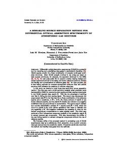
2.1. The Geometrical Model Given the position of the speakers and the microphones, the distances between the ith microphone and the jth speaker dij , and hence the associated propagation times τij , can be calculated (see Figure1 for a simple two-speaker two-microphone case). Accordingly, in a homogenous medium such as air, the attenuation of the received speech signals is related to the distances via αij =

κ d2ij

(5)

where κ is a constant representing the attenuation per unit length in a homogenous medium. Similarly, τij in terms of the number of samples, is proportional to the sampling frequency fs , sound velocity C in air, and the distance dij as: τij =

fs dij C

(6)

which is independent of the directionality. However, in practical situations the speaker’s direction introduces another variable into the attenuation measurement. In the case of electronic loudspeakers (not humans) the directionality pattern depends on the type of loudspeaker. Here, we approximate this pattern as cos(θij /r) where r > 2, which has a smaller value for highly directional speakers and vice versa (an accurate profile can be easily measured using a sound pressure level (SPL) meter). Therefore, the attenuation parameters become κ (7) αij = 2 cos(θij /r) dij If, for simplicity, only the direct path is considered the mixing filter has the form: ˆ H(t)



=

α11 δ(t − τ11 ) α12 δ(t − τ12 ) α21 δ(t − τ21 ) α22 δ(t − τ22 )



(8)

where (ˆ.) denotes the approximation in this assumption. In the fre-

2.2. Initialization for Starting Point ˆ With the help of the estimate H(ω) from the above model, as an initialization of the algorithm in [14] when sources are at the starting point, we improve the convergence of the algorithm and also increase the separation performance together with mitigate the permutation problem. ˆ As such we use H(ω) to provide the initialization for each frequency bin ˆ W1 (ω) = Q1 (ω)H(ω) (10) where Q(ω) is the whitening matrix [15] of the mixtures at the startˆ ing point. Before starting the process H(ω) is normalized once usˆ ˆ ˆ ing H(ω) ← H(ω)/k H(ω)k F where k.kF denotes the Frobenius norm. ˆ The algorithm convergence depends on the estimate of H(ω), to ˆ improve accuracy. In the case of a reverberant environment, H(ω) should ideally be the sum of all echo paths, but this is not available in ˆ practice. As will be shown by later simulations, an estimate of H(ω) obtained from (9) can result in a good performance for the proposed algorithm in a moderate reverberant environment. 2.3. Initialization when Sources are Moving Since the unmixing matrix calculated by geometrically based initialized ICA (initialization described in the above section) is permutation free, therefore W = P DH −1 will approximately become W ≈ H −1 , scaling is not a major issue, and normalization during learning [13] can mitigate its effect. The unmixing matrix of the previous bins with the whitening matrix of the current stage mixtures will provide the intelligent initialization for the current bins as −1 WN +1 (ω) = QN +1 (ω)WN (ω)

(11)

where N is block index and (N ≥ 1). The equivalence between frequency domain blind source separation and frequency domain adaptive beamforming is already confirmed in [16]. We highlight that the whitening matrix Q(ω) has strong impact in such smart initializations. 3. PROPOSED INTELLIGENT INITIALIZATION BASED FASTICA ALGORITHM

Fig. 1. A two-speaker two-microphone setup for recording within a reverberating (room) environment; only distances and angles between sources and microphones are shown. quency domain the above filter has the form ˆ H(ω)



=

α11 e−jωτ11 α21 e−jωτ21

α12 e−jωτ12 α22 e−jωτ22



(9)

201

With the help of the above initializations we increase the separation performance together with mitigate the permutation problem. Crucially, in the proposed IIFastICA approach, since the algorithm essentially fixes the permutation at each frequency bin, there will be no problem while aligning the estimated sources for reconstruction in the time domain. As an initial step, it is usual in ICA approaches to sphere or whiten the data z(ω) = Q(ω)x(ω) (12)

Next when sources are at the starting point we use the column vectors of W1 (ω) obtained from (10), one-by-one, to initialize the fixed point algorithm [14] for each frequency bin. Once the sources start moving we initialize similarly with the column vectors of WN +1 (ω), obtained from (11). Its important to mention that if there was a severe change in the video scene, the initialization for a starting point would be re-applied. Since z(ω) is zero mean, unit variance, with uncorrelated real and imaginary parts of equal variances, the optima of E{G(|wH (ω) z(ω)|2 )} under the constraint E{|wH (ω)z(ω)|2 } = kw(ω)k2 = 1, where E{.} denotes the statistical expectation, (.)H Hermitian transpose, k.k Euclidian norm, |.| absolute function; and G(.) is a nonlinear contrast function, according to the Khun-Tucker conditions satisfy ∇E{G(|wH (ω)z(ω)|2 )} − β∇E{|wH (ω)z(ω)|2 } = 0

(13)

where the gradient denoted by ∇, is computed with respect to the real and imaginary parts of ω separately. The Newton method is used to solve this equation for which the total approximative Jacobian [14] is H

J = 2(E{g(|w (ω)z(ω)| ) + |w (ω)z(ω)|

2

g´(|wH (ω)z(ω)|2 )} − β)I

(14)

which is diagonal and therefore easily invertible, where I denotes the identity matrix and g(.) and g´(.) denote the first and second derivative of the contrast function. We have the following approximative Newton iteration for each vector of each frequency bin wi+ (ω) = E{z(ω)(wi (ω)H z(ω))∗ g(|wi (ω)H z(ω)|2 )} H

2

H

−E{g(|wi (ω) z(ω)| ) + |wi (ω) z(ω)|

wi+ (ω) kwi+ (ω)k

Σi Σω |Hii (ω)|2 h|si (ω)|2 i Σi Σi6=j Σω |Hij (ω)|2 h|sj (ω)|2 i

(17)

where Hii and Hij represents respectively, the diagonal and offdiagonal elements of the frequency domain mixing filter, and si is the frequency domain representation of the source of interest. 4.2. Performance Index (PI) and Evaluation of Permutation The PI as a function of the overall system matrix G = WH is given as P I(G) = +

n X m h1 X

n

i=1

k=1

i abs(Gik ) −1 maxk abs(Gik )

m X n h1 X

m

i=1

k=1

i abs(Gik ) −1 maxi abs(Gik )

(18)

where Gik is the ikth element of G. As we know the above PI based on [3] is insensitive to permutation. We therefore introduce a criterion for the two sources case which is sensitive to permutation and shown for the real case for convenience, i.e. in the case of no permutation, H = W = I or H = W = [0, 1; 1, 0] then G = I and in the case of permutation if H = [0, 1; 1, 0] then W = I and vice versa; therefore, G = [0, 1; 1, 0]. Hence for a permutation free FDCBSS [abs(G11 G22 ) − abs(G12 G21 )] > 0. 5. EXPERIMENTAL RESULTS

2

g´(|wi (ω)H z(ω)|2 )}wi (ω) wi (ω) =

SIR =

(15)

Moving Camera

Room Layout

Fixed Camera

6cm Mic2 1.0 m

Mic1

1.5 m

30

B

o

wm (ω) ← wm (ω) −

H {wm (ω)wj (ω)}wj (ω)

(16)

C

A

E

2

1.0m

j=1

Sp

D Sp ea ke r

ea

1.5m

m−1 X

ke

r1

which importantly eliminates the need to calculate β. where (.)∗ denotes the complex conjugate. In the experiments the statistical expectation is realized as a sample average. Since we have m independent components, the other separating vectors, i.e. wi (ω), i = 2, · · · , m, are calculated in a similar manner and than decorrelated in a deflationary orthogonalization scheme. The deflationary orthogonalization for the m-th separating vector [15] takes the form

The simulations were performed on real recorded speech signals generated for a room geometry as illustrated in Figure 2. As in [13], ˆ the estimate of H(ω) was calculated on the basis of geometrical information obtained from video cameras, when speaker1 was at position A and speaker2 was at position C.

o

2

The SIR is calculated as in [13]

60

H

4.1. Signal-to-Interference Ratio (SIR)

Room = [5.0, 5.0, 5.0]

Finally, after separating all vectors of each frequency bin, we formulate Wj (ω) = [w1 (ω), · · · , wm (ω)] and j = 1, · · · , N . 4. PERFORMANCE MEASUREMENT

Fig. 2. A two-speaker two-microphone layout for recording within a reverberant (room) environment. Speakers move with the speed of 10 deg/sec. Room impulse response length is 130 ms.

In BSS, objective evaluation is generally only possible if true system parameters are known, this is feasible only in artificially mixed data but it is not possible in real BSS experiments since the exact impulse response of the room is not known. In this paper, the performance of the algorithms is first evaluated on the basis of two criteria:

The other important parameters are: block length Tb = 1 sec, FFT length T = 1024, filter length Q = 512 half of T and 50% overlapping was used. The room impulse response duration was 130 ms. Speaker1 moved from A to B i.e. 60 degrees counterclockwise and Speaker2 moved from C to E via D in a back and forth motion i.e.

202

2

(a)

(b)

1

(a)

(b)

(c)

Performance Index (PI)

0.5 0

0

100

200

300

400

(c)

500

0 [abs(G11*G22) − abs(G12*G21)]

30 degrees in total at a speed of 10 deg/sec. This could correspond to moving around a circular table in a tele-conferencing context. We also highlight that to reduce the complexity of the tracker we have assumed radial motion in this work. In our proposed algorithm we select G(y) = log(b + y), with b = 0.1. The resulting performance indices are shown in Figure 3. Figure 3(a) shows good performance i.e. close to zero across the majority of the frequency range, since this is due to the geometrical based initialization mentioned in Section 2.2. In Figures 3(b) and 3(c) the performance is again good but slightly degraded because the estimates for initialization are slightly more biased as explained in Section 2.3.

−2

100

200

300

400

500

0

100

200

300

400

500

0

100

200 300 Frequency bin

400

500

2 0 −2

2 0 −2

1

0

0.5 0

0

100

200

300

400

500

Fig. 4. Evaluation of permutation in each frequency bin at time = 2, 7 and 13 seconds when (a) Both sources are static (b) One source is moving, and (c) Both sources are moving respectively. [abs(G11 G22 ) − abs(G12 G21 )] > 0 means no permutation.

1 0.5 0

0

100

200 300 Frequency bin

400

500

Fig. 3. Performance Index at each frequency bin at time = 2, 7 and 13 seconds when (a) Both sources are static (b) One source is moving, and (c) Both sources are moving respectively. A lower PI refers to a better separation. Since PI mentioned in Section 4.2 based on [3] is insensitive to permutation, this effect was evaluated on the basis of the criterion mentioned in section 4.2. The results at each frequency bin in Figure 4 confirmed that the proposed algorithm automatically mitigates the permutations due to the intelligent initializations mentioned in Sections 2.2 & 2.3, and therefore no additional processing is required. Figures 4(a) and 4(b) show improved results over 4(c) because when both sources are moving there is more variation in the mixing environment, in spite of the strong impact of Q(ω) as mentioned in section 2.3 the initialization is slightly more biased, therefore as we will explain in the next paragraph, the algorithm generally requires more iterations to converge when sources are moving. Since the convergence rate of any algorithm has a vital rule for a real time system. The number of iterations required for the convergence of the underlying cost, in the proposed IIFastICA algorithm at different conditions of the sources is shown in Table 1. The maximum of seven iterations when both sources are moving confirms that the proposed algorithm is more suitable for a real-time system.

203

The performance indices and evaluation of permutation by the original FastICA algorithm [14] with random initialization, on the recorded mixtures when both sources were static, are shown in Figure 5. As shown in Table 1, twenty five iterations are required for the performance level achieved in Figure 5(a) with no solution for permutation as shown in Figure 5(b). The permutation problem in frequency domain BSS degraded the SIR to approximately zero on the recorded mixtures. Table 1. Number of iterations required for convergence in the proposed IIFastICA algorithm and the Bingham and Hyvrinen FastICA algorithm [14], averaged over all frequency bins under different conditions of the sources. Sources Condition Iterations Iterations (IIFastICA) ([14]) Both sources are static 4 25 One source is moving 5 N/A Both sources are moving 7 N/A The SIR as mentioned in Section 4.1 was next calculated. The separation was performed at Tb = 1 sec, and Figure 6 confirms that average SIR-Improvement when both speakers were stationary is 20 dB, when one speaker was moving 17 dB and when both speakers were moving 14.5 dB. The minimum 14.5 dB SIR-Improvement again confirmed that no additional postprocessing is required which has been confirmed subjectively by listening tests.

(b)

[abs(G11*G22) − abs(G12*G21)]

(a)

Performance Index (PI)

7. REFERENCES [1] S. Haykin and Ed.., Unsupervised Adaptive Filtering (Volume I: Blind Source Separation), John Wiley, New York, 2000.

1

[2] A. S. Bregman, Auditory Scence Analysis, MIT Press, Cambridge, MA, 1990.

0.5

0

0

100

200 300 Frequency bin

400

[3] A. Cichocki and S. Amari, Adaptive Blind Signal and Image Processing: Learning Algorithms and Applications, John Wiley, 2002.

500

2 1

[4] W. Wang, S. Sanei, and J.A. Chambers, “Penalty function based joint diagonalization approach for convolutive blind separation of nonstationary sources,” IEEE Trans. Signal Processing, vol. 53, no. 5, pp. 1654–1669, 2005.

0 −1 −2

0

100

200 300 Frequency bin

400

500

Fig. 5. (a) Performance Index at each frequency bin and (b) Evaluation of permutation in each frequency bin, when both sources are static for Bingham and Hyvrinen FastICA algorithm [14]. A lower PI refers to a better separation and [abs(G11 G22 ) − abs(G12 G21 )] > 0 means no permutation.

[6] S. Makino, H. Sawada, R. Mukai, and S.Araki, “Blind separation of convolved mixtures of speech in frequency domain,” IEICE Trans. Fundamentals, vol. E88-A, no. 7, pp. 1640–1655, Jul 2005. [7] C. Cherry, “Some experiments on the recognition of speech, with one and with two ears,” The Journal of the Acoustical Society of America, vol. 25, no. 5, pp. 975–979, September 1953.

20 18

SIR−Improvement (dB)

[5] T. Tsalaile, S. M. Naqvi, K. Nazarpour, S. Sanei, and J. A. Chambers, “Blind source extraction of heart sound signals from lung sound recordings exploiting periodicity of the heart sound,” Proc. IEEE ICASSP, Las Vegas, USA, 2008.

[8] R. Mukai, H. Sawada, S.Araki, and S. Makino, “Robust realtime blind source separation for moving speakers in a room,” Proc. IEEE ICASSP 2003, Hong Kong, April 6-10.

16 14

One source is moving

Both sources are static

12 10

Both sources are moving

[9] A. Koutras, E. Dermatas, and G. Kokkinakis, “Blind source separation of moving speakers in real reverberant environment,” Proc. IEEE ICASSP 2000, pp. 1133–1136.

8 6 4

[10] R. E. Prieto and P. Jinachitra, “Blind source separation for time-variant mixing systems using piecewise linear approximations,” Proc. IEEE ICASSP 2005, pp. 301–304.

2 0

0

2

4

6

8

10

12

14

16

Time (Sec.)

Fig. 6. SIR-Improvement when sources are static, one source is moving and both sources are moving.

[11] S. Haykin and Ed.., New Directions in Statistical Signal Processing: From Systems to Brain, The MIT Press, Cambridge, Massachusetts London, 2007. [12] W. Wang, D. Cosker, Y. Hicks, S. Sanei, and J. A. Chambers, “Video assisted speech source separation,” Proc. IEEE ICASSP, pp. 425–428, 2005.

6. CONCLUSION

A new multimodal approach for FDCBSS, with intelligent initialization for FastICA, for moving sources has been presented in this research work. The advantage of our proposed algorithm was confirmed in simulations from a real room environment. The location and direction information were obtained using a number of cameras equipped with a speaker tracking algorithm and this information was used in the initialization of the proposed algorithm. The proposed algorithm is block-based and the initialization is performed based on either the geometrical information obtained from tracking or the BSS results from the previous block. The separation was evaluated objectively by the performance indices with solution for permutation at frequency bin level and overall SIR-Improvement at different conditions of sources, and also confirmed subjectively by listening tests. The outcome of this approach is a step towards solving the cocktail party problem for moving sources by using a cognitive approach.

204

[13] S. Sanei, S. M. Naqvi, J. A. Chambers, and Y. Hicks, “A geometrically constrained multimodal approach for convolutive blind source separation,” Proc. IEEE ICASSP, pp. 969–972, 2007. [14] E. Bingham and A. Hyvrinen, “A fast fixed point algorithm for independent component analysis of complex valued signals,” Int. J. Neural Networks, vol. 10, no. 1, pp. 1–8, 2000. [15] A. Hyvrinen, J. Karhunen, and E. Oja, Independent Component Analysis, New York: Wiley, 2001. [16] S.Araki, S. Makino, Y. Hinamoto, R. Mukai, T.Nishikawa, and H. Saruwatari, “Equivalence between frequency domain blind source separation and frequency domain adaptive beamforming for convolutive mixtures,” EURASIP J. Appl. Signal Process., , no. 11, pp. 1157–1166, 2003.