A Least-Squares Approach to Blind Source Separation in Multispeaker

59

JOURNAL OF COMPUTERS, VOL. 2, NO. 7, SEPTEMBER 2007

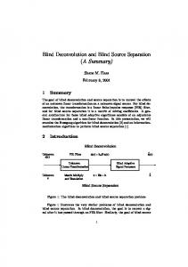
A Least-Squares Approach to Blind Source Separation in Multispeaker Environments Robert M. Nickel and Ananth N. Iyer Department of Electrical Engineering, The Pennsylvania State University, University Park, PA 16802, USA Email: {rmn10, ani103}@psu.edu Abstract— We are proposing a new approach to the solution of the cocktail party problem (CPP). The goal of the CPP is to isolate the speech signals of individuals who are concurrently talking while being recorded with a properly positioned microphone array. The new approach provides a powerful yet simple alternative to commonly used methods for the separation of speakers. It relies on the existence of so called exclusive activity periods (EAPs) in the source signals. EAPs are time intervals during which only one source is active and all other sources are inactive (i.e. zero). The existence of EAPs is not guaranteed for arbitrary signal classes. EAPs occur very frequently, however, in recordings of conversational speech. The methods proposed in this paper show how EAPs can be detected and how they can be exploited to improve the performance of blind source separation systems in speech processing applications. We consider both, the instantaneous mixture and the convolutive mixture case. A comparison of the proposed method with other popular source separation methods is drawn. The results show an improved performance of the proposed method over earlier approaches. Index Terms— blind source separation, least-squares optimization, cocktail party problem, exclusive activity periods.

I. I NTRODUCTION An illustration of the scenario considered in the cocktail party problem (CPP) is shown in figure 1. We are recording an acoustic scene with an array of microphones. If we want to isolate the voice of a single speaker out of a mixture of signals from different sources then it is implicitly necessary to estimate the transmission properties (or equivalently the inverse transmission properties) of all channel between all microphones and all sources. Up to date, the most successful approaches to solving the cocktail party problem (CPP) employ blind source separation (BSS) techniques based on an assumption of statistical independence of the sources [1], [2]. The goal is to find an un-mixing system that maximizes a “measure of independence” from the reconstructed source signals. Generally, one distinguishes between methods that consider instantaneous mixing and methods that address convolutive mixing [1]–[3]. This paper is based on “A Novel Approach to Automated Source Separation in Multispeaker Environments,” by R. M. Nickel and A. N. Iyer, which appeared in the Proceedings of the IEEE International Conference on Acoustics, Speech, and Signal Processing (ICASSP), vol. c 2005 IEEE. 5, pp. 629-632, May 14-19, 2006, Toulouse, France.


© 2007 ACADEMY PUBLISHER

Figure 1. An illustration of the scenario considered in the cocktail party problem. In order to isolate the speech signal of a targeted speaker we need to implicitly estimate the transmission channels between all sources and all microphones.

The crux of the aforementioned approach is to find a good (and mathematically tractable) “measure for independence.” It was shown that a suitable objective in finding a solution is provided by the minimization of a contrast function which is a function of the PDF of the observed signals [2], [4]. In the context of speech and audio signal processing a suitable contrast function is usually derived from a likelihood measure and/or the INFOMAX concept [5]. The optimization procedure that minimizes a contrast function (and thus provides a solution to the BSS problem) is generally called an independent component analysis (ICA) [2]. Even though the BSS techniques have achieved remarkable results in the separation of mixed audio signals, they are still suboptimal in regard of separation of speech, partially because they usually do not permit an exploitation of the highly structured nature of speech. Solutions to the more general convolutive mixture case are significantly more complicated than solutions to the instantaneous mixture case [6]–[10]. Most solutions can be classified as either, time domain approaches (see [11] and the references therein) or frequency domain approaches (see [1], [12], [13]). More specifically, we have to distinguish between: the domain in which we model the mixing process (mixing domain) and the domain in which we model the statistics of the source signals (source domain). A choice of either time or frequency for each of these domains have significant advantages and disadvantages (see [1]).

60

JOURNAL OF COMPUTERS, VOL. 2, NO. 7, SEPTEMBER 2007

In this paper we are developing an alternative approach based on a concept introduced by Huang, Benesty, and Chen in 2005 [14]. The alternative approach does not explicitly rely on an independence assumption between sources. Instead, we are assuming the existence of exclusive activity periods (EAPs). EAPs are time intervals during which only one source is active and all other sources are silent. The existence of EAPs is not guaranteed for arbitrary signal classes, but EAPs occur very frequently in recordings of conversational speech. The caveat of the newly proposed method is that one needs to reliably detect exclusive activity periods from the observed signals. The detection of such periods becomes possible if we are focusing on the unique structure of speech signals and in particular the unique structure of voiced segments of the speech signals. The technical details of the proposed methodology are presented in sections II and III. Section II focuses on the instantaneous mixing case and section III focuses on the convolutive mixing case. An experimental verification and performance analysis is presented in section IV. The results are discussed in sections V and VI. II. I NSTANTANEOUS M IXING The considered scenario is described by the following mathematical model: we have K speakers in a room, each of which produces a speech signal xk [n] (for k = 1, 2, . . . , K). The K speech signals are captured by M microphones (M ≥ K), each of which must be placed such that the acoustic waveforms measured must be significantly different from microphone to microphone1 . The signal recorded at microphone m will be referred to as the observed signal and is denoted as ym [n] (for m = 1 . . . M ). To streamline the notation it is beneficial to introduce the following vectors: xk ym

= =

[ xk [1] xk [2] . . . xk [P ] ]T [ ym [1] ym [2] . . . ym [P ] ]T ,

(1) (2)

where P is the observation segment length in samples. For simplicity we will use the notation xk and ym in three ways: (i) to indicate vectors that encompass the entire recording length, (ii) to indicate one of a successive set of 40 msec long segments of the recording, and (iii) to indicate an exclusive activity period which spans multiple successive segments of length 40 msec. Matrices are formed from the vectors as X = [ x1 x2 . . . xK ]T and Y = [ y1 y2 . . . yM ]T . If we assume instantaneous mixing then the connection between the source signal matrix X and the observed signal matrix Y is determined by the constant mixing matrix A: Y = A · X.

(3)

In general, the solution to the CPP is defined so as to determine an inverse/de-mixing matrix W such that ˆ from matrix X ˆ =W·Y X (4) 1 Appropriate placement of the microphones is crucial to ensure that the resulting estimation problem is not being ill-conditioned.

© 2007 ACADEMY PUBLISHER

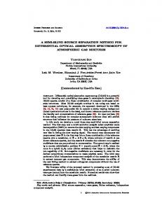
Figure 2. A block diagram of the proposed source separation algorithm. The de-mixing matrix W is estimated from EAP sections of the observed signals Y. The ˆ are obtained from equation (4). source estimates X

provides an estimate for the rows of matrix X. The matrix W is considered a de-mixing matrix when the matrix product W · A is a permutation matrix. The proposed source separation algorithm consists of two main parts: i) the detection of EAP segments and ii) the determination of the de-mixing matrix W. A block diagram of the proposed algorithm is shown in figure 2. A. EAP Detection The detection of EAPs is facilitated by the following definition of a normalized signal-to-interference ratio (SIR) γ: 
xTk xk 1 −1 . (5) γ = K−1 max K K T k i=1 xi xi If we let the xk ’s denote successive 40 msec long segments of the source signals then we obtain an SIR measure γ for each segment. Note that the SIR is normalized such that 0 ≤ γ ≤ 1 (with γ = 1 indicating a perfect EAP event). Unfortunately, we cannot access the true underlying SIR since we cannot measure the source signals xk directly. Instead, we are estimating γ from the observations ym . The proposed estimator is based on the following three features: (i) A Periodicity Measure. The pitch determination algorithm (PDA) developed by Medan et. al. [15] aims to determine the pitch of a voiced speech segment. The method involves computing normalized inner products between adjacent, variable length speech segments. The inner product is maximized when the segment length equals the pitch period. The normalized inner product at the pitch provides a measure of periodicity fp for the given signal segment ym . (ii) The Harmonic-to-Signal Ratio. The energy of a voiced speech segment is concentrated around the harmonic frequencies of its pitch. The harmonicto-signal ratio (HSR) fh is defined as the ratio of spectral energy around the pitch harmonics versus the overall energy of signal ym . Its computation is achieved by comparing the energy of the output of a pitch synchronous comb-filter with the total signal energy [16].

JOURNAL OF COMPUTERS, VOL. 2, NO. 7, SEPTEMBER 2007

61

(iii) The Spectral Autocorrelation. Spectral autocorrelation measures are used in many PDAs (in addition to temporal correlation measures) to combat pitchdoubling/pitch-halving errors. We are employing the normalized spectral autocorrelation proposed in [16]. The maximum autocorrelation value fs in the pitch frequency range (50Hz to 500Hz) is determined and used as a feature for the SIR estimation. The SIR is estimated via γˆ = Φ(fp , fh , fs ) in which Φ(. . .) is a three dimensional, second order polynomial. The optimal polynomial coefficients are chosen to minimize the least-squares error between the estimated SIR (ESIR) γˆ and the true underlying SIR γ for the training set described in section IV. The resulting normalized correlation coefficients between fp , fh , fs , γˆ and γ are shown in table I. The EAP detection is performed with a threshold test. A segment is flagged as an EAP if γˆ is greater or equal to a threshold γ¯ (see section IV). A time segment is considered an exclusive activity period if the corresponding segments ym are all flagged as EAPs across all channels m = 1 . . . M . TABLE I. C ORRELATION C OEFFICIENTS FOR SIR E STIMATION Feature Periodicity Measure fp Harmonic-to-Signal Ratio fh Spectral Autocorrelation fs Polynomial Estimate γ ˆ

Correlation with γ 0.5838 0.4360 0.4329 0.6338

During a true exclusive activity period it is readily verified that the observed signals yi are scalar multiples of the one active source signal xq . We can obtain an estimate for xq from each channel i by multiplying the channel output yi with a channel specific scalar wi : (6)

ˆ qj for all i and j, which leaves ˆ qi = x Ideally, we want x us with an infinite number of choices for the wi’s if all of the yi’s are truly linearly dependent. Due to imperfect EAP detection and background noise, however, we are ˆ qj for all i and j for ˆ qi = x generally not able to achieve x any set of channel weights wi . Instead, we may seek to ˆ qi choose the wi’s such that the deviation between each x M q 1 q ˆ j is minimized, i.e. ¯ = M j=1 x and their average x minimize C q = wi

M 

ˆ qi − x ¯ q 2 subject to  x ¯ q 2 = ζ 2 . x

i=1

(7) The constraint is necessary to avoid the trivial (yet meaningless) solution wi = 0 for all i. Expanding the terms of the cost function leads to Cq =

M  i=1

wi2 yiT yi −

M M 1  wi wk yiT yk , M i=1

© 2007 ACADEMY PUBLISHER

k=1

C q = wT [ Rd −

1 MR]w

(9)

with R = YT Y, Rd = diag(R) and w = [ w1 , w2 , . . . , wM ]T . With Lagrange multiplier λ we can cast equation (7) into the Lagrange function L(w, λ) = wT [ M Rd − (1 + λ) R ] w − λ M 2 ζ 2 . (10) Differentiating L(w, λ) with respect to w and equating to zero results in the condition Rd w =

λ+1 M

R w.

(11)

Condition (11) is satisfied by the generalized eigenvectors of matrices R and Rd (with λ+1 M being the generalized eigenvalues). It is readily shown that out of the M generalized eigenvectors we must choose the one wq with the smallest eigenvalue to minimize the cost function C q . The transpose of the solution wq establishes the q’s row of the de-mixing matrix W. We must observe at least one EAP from every source to obtain a full estimate of W. The decision of whether a set of disjoint EAPs belongs to the same source or to different sources is done with a simple hierarchical clustering algorithm2 . If multiple estimates of wq (from disjoint EAPs) are cast into the same cluster then their (renormalized) centroid is used as the corresponding row in W. III. C ONVOLUTIVE M IXING

B. Estimation of the De-mixing Matrix

ˆ qi = wi yi . x

which can be compactly written in matrix notation as

(8)

The methods proposed in the previous section for the instantaneous mixing case are readily generalized to the convolutive mixing case. A block diagram that depicts the considered scenario is shown in figure 3. For simplicity we assume that we have M unknown source signals xi [n] for i = 1 . . . M . The transmission path between source i and receiver j is described by the transfer function of a linear time-invariant system with impulse response gij [n]. The resulting M observation signals yj [n] are generated according to:  ∞ M   gij [k] xi [n − k] for j = 1 . . . M. yj [n] = i=1

k=0

(12) Equation (12) can also be expressed in the z-domain as Y(z) = G(z) · X(z),

(13)

in which X(z) is the z-transform of multichannel signal x[n] = [ x1 [n] x2 [n] . . . xM [n] ]T , Y(z) is the z-transform of multichannel signal y[n] = [ y1 [n] y2 [n] . . . yM [n] ]T , and G(z) is a matrix with the z-transforms of the impulse responses gij [n] for all i and j. The goal in convolutive blind source separation is to ˆ find a matrix of transfer functions H(z) such that X(z) given by ˆ X(z) = H(z) · Y(z) (14) 2 It is assumed that the underlying number of sources is known and that all sources have at least one EAP.

62

JOURNAL OF COMPUTERS, VOL. 2, NO. 7, SEPTEMBER 2007

General Model Scenario Sources

Mixture Model

periodic signals yield correlation values less than one. As a consequence, we can define a short-time periodicity measure as:

Observations

x1 [n]

gii [n]

y1 [n]

x2 [n]

gij [n]

y2 [n]

STPMj [n] =

gjj [n]

yM[n]

Figure 3. A block diagram of the mixing scenario described by equation (12). The M unknown signal sources are labelled with xi [n] (for i = 1 . . . M ). The M observations are labelled with yj [n] (for j = 1 . . . M ).

pmin = Fs / 500 Hz

A. EAP Estimation for Convolutive Mixtures of Speech An exclusive activity period is a time during which only one source xi [n] is active and all other sources xk [n] are silent, i.e. xk [n] = 0 for k = i. Similarly to the instantaneous mixing case, the estimation of exclusive activity periods for speech sources xi [n] can be based on the (almost) periodic nature of vocalic sounds. If only a single person is speaking then all observations yj [n] exhibit time intervals with a periodic structure. When multiple persons are speaking the periodicity is generally destroyed [17]. Again, we use a modification of the robust shorttime periodicity measure proposed Medan et al. [15] (see section II-A). They consider the similarity between two adjacent observation segments of length k: sj1 [n, k] =[ yj [n − k] . . . yj [n − 2] yj [n − 1] ]T (15)

sj2 [n, k] =[ yj [n] yj [n + 1] . . . yj [n + k − 1] ]T . (16) A correlation measure NCORj [n, k] is defined through a normalized inner product of vectors sj1 [n, k] and sj2 [n, k]: sj1 [n, k]T sj2 [n, k]

 sj1 [n, k]  ·  sj2 [n, k] 

.

(17)

The normalization ensures that the correlation measure is bounded between zero and one, i.e. 0 ≤ NCORs [n, k] ≤ 1. The correlation measure is equal to one at the true period p of a perfectly periodic signal. Less than perfectly © 2007 ACADEMY PUBLISHER

(18)

and

pmax = Fs / 50 Hz . (19)

A second feature that correlates well with EAPs is the so called short-time zero crossing rate [16]:

is (in some appropriate metric) as close to X(z) as possible. Similarly to the method described in section II we are applying the following three-step approach: 1) Find a set of time intervals [n1 , n2 ] during which only one source is active and all other sources are silent, i.e. find all exclusive activity periods (EAPs). 2) Find a set of transfer functions that deconvolve the sources during EAPs. 3) Construct H(z) by combining the results from different EAPs from different sources. One of the caveats of the proposed approach is that EAP detection is slightly more complicated with convolutive mixtures than it is with instantaneous mixtures. We have to revise our EAP detection method first.

NCORj [n, k] =

{ NCORj [n, k] } .

The search range for the maximum should be bounded by the typical pitch range of human speech (50Hz...500Hz). For observation signals that are sampled with sampling frequency Fs we have:

gji [n] xM[n]

max

pmin ≤k≤pmax

STZCj [n] =

n+L 

| sign(yj [m]) − sign(yj [m − 1]) |.

m=n−L

(20) In our notation sign(x) is equal to +1 for x ≥ 0 and −1 for x < 0. The zero crossing rate counts the number of transitions from positive samples to negative samples within the range (n − L − 1) . . . (n + L). The range length is usually chosen as L = Fs · 10 msec. Typically, the zero crossing rate is low for EAP sections and high otherwise. For the STZC measure to work properly it is important that possible quantization offsets in the recorded speech signal are removed prior to processing. A normalized short-time zero crossing measure NZCMj [n] is constructed with the maximum ZCmaxj and the minimum ZCminj of STZCj [n] over all n: NZCMj [n] =

STZCj [n] − ZCmaxj . ZCmaxj − ZCminj

(21)

The identification of EAP candidates is done as follows: 1) find all times n for which STPMj [n] ≥ 0.7 for all observations j = 1 . . . M , 2) expand the so found sections in forward and backward direction until STPMj [n] < 0.6, 3) remove times for which NZCMj [n] > −0.5, and 4) retain only the intersection of all EAP candidates across all channels j = 1 . . . M . An example for STPMj [n], NZCMj [n], and the resulting set of EAP candidate sections is shown in figure 6. B. Blind EAP Deconvolution In this section we discuss the subproblem of blind system identification under an exclusive activity assumption, i.e. we assume that we have identified a time interval [n1 , n2 ] during which only source xi [n] is active and all other sources are silent, i.e. xk [n] = 0 for k = i. Under the EAP assumption we may attempt to reconstruct source xi [n] from each observation yj [n] via an appropriately ˆ ij [n]: chosen inverse filter h x ˆji [n] =

P 

ˆ ij [k] yj [n − k]. h

(22)

k=0

ˆji [n] for all j = 1 . . . M . Practically, Ideally xi [n] = x ˆji [n] for k = j due to noise, however, we have x ˆki [n] = x

JOURNAL OF COMPUTERS, VOL. 2, NO. 7, SEPTEMBER 2007

imperfect estimation of the EAPs, improper choice of P , non-minimum phase properties of gij [n], and so forth. An estimate Ei of the reconstruction error can be defined with Ei =

M  

|x ˆji [n] − x ¯i [n] |2

(23)

M 1  j x ˆ [n]. M j=1 i

(24)

j=1 n

and

x ¯i [n] =

It is readily seen from equation (23) that a perfect ˆji [n] yields a minimum error reconstruction with xi [n] = x ˆji [n] may not estimate of Ei = 0. Unfortunately, xi [n] = x be the only solution that satisfies Ei = 0 (e.g. if the gij [n] are linearly dependent). One may hope, however, that (if the gij [n] are sufficiently different) a global minimization ˆ ij [n] for of Ei will lead to good estimates for the h j = 1 . . . M. The computation of the global minimum of Ei is aided by the following notation. We define:   ˆji [n1 + P ] . . . x ˆji [n2 − 1] x ˆji [n2 ] , x ˆji = x ⎡ ⎢ ⎢ Y =⎢ ⎢ ⎣ j

and

⎤ yj [n1 + P ] ⎥ .. ⎥ . yj [n1 + 1] yj [n1 + 2] · · · ⎥, ⎥ .. .. .. .. ⎦ . . . . ··· ··· yj [n2 ] yj [n2 − P ]   ˆ ij [1] h ˆ ij [0] . ˆ ij [P ] . . . h ˆj = h h (25) i yj [n1 ]

yj [n1 + 1]

···

ˆ j and: Equation (22) can be rewritten as x ˆji = Yj h i x ¯i =

M M 1  j 1  j ˆj x ˆi = Y hi . M j=1 M j=1

The error estimate (23) becomes:  2 M M      j ˆj k ˆk  1 Ei = Y hi   Y hi − M   j=1

=

M 

(26)

(27)

k=1

ˆj ] Yj h ˆj − [ Yj h i i

j=1

M M 1  ˆ ki ] Yj h ˆj . [ Yk h i M j=1 k=1

We define the matrices Rjk = [ Yk ] Yj and ⎡ ⎤ R11 R12 · · · R1M ⎢ ⎥ .. ⎢ R21 R22 · · · ⎥ . ⎥, RF = ⎢ ⎢ . ⎥ . . .. .. .. ⎣ .. ⎦ . RM 1 · · · · · · RM M ⎤ ⎡ R11 0 ··· 0 ⎥ ⎢ .. ⎥ ⎢ 0 . R22 · · · ⎥, RD = ⎢ ⎥ ⎢ . . .. .. ⎦ ⎣ .. . 0 0 ··· 0 RM M   ˆ 1i ] [ h ˆ 2i ] . . . [ h ˆM ˆi = [h and H ] . i © 2007 ACADEMY PUBLISHER

(28)

(29)

(30)

63

Using equations (25) to (30) we can compactly write the error estimate as ˆ i [ RD − 1 RF ] H ˆ i. (31) Ei = H M In order to avoid the trivial minimization of equation (31) ˆ i = 0) we constrain the solution to (with H 1 ˆ F ˆ x ¯i 2 = 2 H (32) i R Hi = 1. M We have thus reformulated the problem into that of ˆ i that minimizes Ei subject to equafinding the vector H tion (32). It is readily shown with Lagrange multipliers that the solution to the above problem is provided by one of the generalized eigenvectors Φm of matrices RD and RF : ϕm RD Φm = RF Φm .

(33)

We assume that the eigenvalues ϕm are sorted in decreasing order ϕ1 ≥ ϕ2 ≥ ϕ3 ≥ ϕ4 ≥ . . . and that the eigenvectors are normalized such that  Φm  = 1 for all m. Choosing Φm as the solution leads to an error estimate of Ei = M ( ϕMm − 1). The optimal solution, i.e. the one that minimizes Ei is thus given by ˆ i = Φ1 H

and

Ei = M (

M − 1). ϕ1

C. Blind Source Separation As a result of the methods described in sections IIIˆi A and III-B we obtain an inverse filter estimate H (with its associated eigenvalue ϕ1 ) for each separately identified EAP section. In a first step we discard all EAP ˆ i ) for which log10 M sections (and H M −ϕ1 was greater than a certain EAP acceptance threshold (EAT - see section V). In a second step we use a simple minimum Euclidean distance hierarchical clustering method [18] ˆ i to one of the M sources. All to associate each vector H vectors associated with the same source k are averaged3 ¯ k for (arithmetic mean) into an average eigenvector H each source k = 1 . . . M . By extracting the corresponding ¯ j in analogy to equation (30): subvectors h i   ¯ 1i ] [ h ¯ 2i ] . . . [ h ¯M ¯ Hi = [ h , (34) i ] ¯j : we obtain a complete set of inverse filter vectors h i   j ¯ ij [P ] . . . h ¯ ij [1] h ¯ ij [0] . ¯ = h h (35) i An estimate for the mixing matrix G(z) from equation (13) is obtained from:   1 ˆ G(z) = P , (36) −k ¯ ij k=0 hij [k] z where notation [G]ij refers to the element of matrix G in row i and column j. An estimate for the demixing matrix H(z) from equation (14) can be obtained by numerically ˆ inverting G(z) via Gaussian elimination [19]. Unfortunately, the inversion process may introduce unstable poles 3 The weight for each vector was chosen proportional to the number of samples contained in the associated EAP section. Longer EAP sections had thus more weight then shorter ones.

64

JOURNAL OF COMPUTERS, VOL. 2, NO. 7, SEPTEMBER 2007

ˆ into the transfer functions of H(z). The production of stable filters can be enforced by mirroring poles that fall outside of the unit circle back into the inside of the unit circle. The mirroring process distorts the correct phase response, but leaves the magnitude response of individual channels intact.

110

100 95 SNR [dB]

IV. E XPERIMENTS

105

We evaluated the performance of the proposed method with mixing/de-mixing trials over speech data from the TIMIT4 database. The TIMIT dataset contains recordings of 10 phonetically rich sentences from 630 speakers of 8 major dialects of American English. The corpus is stored in 16bit/16kHz waveform files for each utterance. One subset of files is strictly reserved for training and another subset is reserved for testing.

90 85 80 75 70 65

0.5

0.6

4 The TIMIT database is available through the Linguistic Data Consortium (LDC) at the University of Pennsylvania (www.ldc.upenn.edu).

© 2007 ACADEMY PUBLISHER

1

Source Signals

Channel #1

1 0.5 0 −0.5 −1 0

0.5

1

1.5

2 2.5 Time [sec]

3

3.5

4

0.5

1

1.5

2 2.5 Time [sec]

3

3.5

4

Channel #2

1 0.5 0 −0.5 −1 0

[i,j]∈P

Figure 5. An example of two source signals x1 [n] and x2 [n] from the TIMIT database. The signals were aligned to have a 30% overlap in time. Mixed Signals and Features

Channel #1

1 0.5 0 −0.5 −1 0

0.5

1

1.5

2 2.5 Time [sec]

3

3.5

4

0.5

1

1.5

2 2.5 Time [sec]

3

3.5

4

1 Channel #2

(37) ˆ i ) to ˆ Ti xj /(ˆ xTi x The scaling factor η is chosen as η = x account for the unknown scaling of the reconstructed signals. Parameter P refers to a set of M index pairs [i, j] with i = 1 . . . M and j = 1 . . . M and such that each number between 1 and M is only used once for i and once for j. P is the entirety of all possible index sets P. The minimization over P accounts for the unknown signal permutations introduced by WA as discussed in section 2. In a first experiment we ran several sets of 256 random mixing/de-mixing trials with M = 2 over the training subset of the corpus. For each set of 256 trials we chose a different EAP decision threshold γ¯ as described in section II. The resulting average SNR (averaged over all trials) as a function of γ¯ is displayed in figure 4. The optimal threshold, i.e. the one that produced the highest average SNR, was found to be γ¯ = 0.85. In a second experiment we ran several sets of 256 random mixing/de-mixing trials over the testing subset of the corpus. This time, we kept γ¯ fixed at 0.85 and varied the number of sources/channels M . The resulting average SNR (averaged over all 256 trials per M ) as a function of M is shown in figure 9 (EAPD).

0.9

Figure 4. Determination of the EAP decision threshold γ¯ . The average SNR is maximized in the two channel case (M = 2) for γ¯ = 0.85.

A. Instantaneous Mixing During each mixing/de-mixing trial we randomly chose M utterances xi from the corpus. The M utterances were mixed with a random mixing matrix A according to equation (3) to produce M observations yi . The elements of A were chosen as independent, uniformly distributed random numbers over the interval [0, 1]. The observations yi were then subjected to the proposed deˆi. mixing procedure to produce M source estimates x The quality of the de-mixing process was measured with the following signal-to-noise ratio (SNR):    xTi xi 10 SNR = min M log . P∈P ˆ j )T (xi − η x ˆj ) (xi − η x

0.7 0.8 SIR Threshold

0.5 0 −0.5 −1 0

Figure 6. The resulting mixed signals y1 [n] and y2 [n] from the example in figure 5. The upper dashed line in each axis indicates the resulting STPMj [n] contour (equation (18)) and the lower dashed line indicates the resulting NZCMj [n] contour (equation (21)). The gray regions indicate the EAP sections that were estimated from the mixed signals.

JOURNAL OF COMPUTERS, VOL. 2, NO. 7, SEPTEMBER 2007

65

Demixed Signals − EAP Method

Channel #1

1 0.5 0 −0.5 −1 0

0.5

1

1.5

2 2.5 Time [sec]

3

3.5

4

0.5

1

1.5

2 2.5 Time [sec]

3

3.5

4

Channel #2

1 0.5 0 −0.5 −1 0

Figure 7. The resulting demixed signals x ˆ1 [n] and x ˆ2 [n] from the example in figure 5 after application of the proposed EAP method. Both signals are very close to the original source signals x1 [n] and x2 [n] depicted in figure 5. Demixed Signals − Parra/Spence Method

Channel #1

1 0.5 0 −0.5 −1 0

0.5

1

1.5

2 2.5 Time [sec]

3

3.5

4

0.5

1

1.5

2 2.5 Time [sec]

3

3.5

4

Channel #2

1 0.5 0 −0.5 −1 0

Figure 8. The demixing result of a commonly used conventional method of blind source separation after L. Parra and C. Spence [20] (see section V).

B. Convolutive Mixing Our experiments with convolutive mixing were conducted over the SI-subset of the TIMIT database. The chosen subset consists of recordings from 630 subjects each uttering 3 phonetically-diverse sentences5 . The signals were low-pass filtered and down-sampled to 8 kHz prior to processing. All 3 sentences from the same speaker were concatenated and then truncated to 4 seconds. As a result we received a total of 630 different 4 seconds long source signals x[n]. We ran experiments with different source numbers (M = 2, 3, and 4) and particularly small filter lengths (P + 1 = 5, 7, and 10). Unfortunately, the increased complexity and the poor conditioning of the underlying matrices RF and RD at higher dimensions prevented 5 None

of the sentences are repeated more than once.

© 2007 ACADEMY PUBLISHER

us (as of now) from considering more realistic filter lengths (between 1000 . . . 100000) of real reverberant environments. The presented theory holds for arbitrary filter lengths, however, one must employ an eigenvector/eigenvalue decomposition algorithm with a sensitivity far beyond the algorithm available to the authors. For each M the available data was randomly split6 into [ 630/M ] groups of M source signals xi [n]. To simulate conversational speech the signals were partially faded out to obtain a relative time-overlap between signals of roughly 30% (see figure 5). The M source signals of each group were mixed with order-P random minimum phase filters gij [n] according to equation (12). The resulting observations yj [n] for j = 1 . . . M were then used to ˆ estimate the inverse filter matrix H(z) according to section III. The reconstructed source signal estimates x ˆi [n] for i = 1 . . . M were computed according to equation (14) ˆ ˆ via X(z) = H(z) Y(z). The quality of the estimated model was evaluated with the Signal-to-Interference Ratio (SIR in [dB]) between the reconstructed signal x ˆi [n] and the original signal xi [n]:    | xi [n] |2 n SIRi = max 10 log10  . p ˆi [n − p] |2 n | xi [n] − x (38) The evaluation of the SIR was performed under careful consideration of possible numbering permutations between the original signals and the reconstructions. Figures 5 to 7 show an example for an experiment with two sources. The gray regions in the figures indicate the EAP sections that were estimated from the mixed signals y1 [n] and y2 [n] from figure 6. Figure 8 shows the result for a commonly used conventional method of blind source separation after L. Parra and C. Spence [20] (see section V). V. R ESULTS The performance results of the proposed EAP method for the instantaneous mixing case are presented in figure 9. The performance of two other popular BSS methods, FastICA7 [21] and AMUSE7 [11], are provided for comparison. For each method the average SNR and the standard deviation over all 256 trials per M are shown (via I-bars). The proposed EAPD method clearly outperforms the other two methods for smaller source numbers. As the number of simultaneously talking sources M increases, the number (and quality) of available EAP sections naturally decreases. As a result, the performance of the proposed method declines. All methods performed around the same average SNR for 6 and more simultaneous sources (with a slight edge of FastICA and EAPD over AMUSE). Increased errors in EAP detection, however, lead to a much larger standard deviation of the EAPD me6 Every

source signal was only used once. employed software provided by the original developers of the FastICA and AMUSE algorithms for the comparison. All third part software was run with default parameters. 7 We

66

JOURNAL OF COMPUTERS, VOL. 2, NO. 7, SEPTEMBER 2007

70 EAPD FICA AMUSE

60

Source Number M 2 2 2 3 3 3 4 4

SBR [dB]

50

40

30

20

10

0 1

2

3

4 5 Number of Sources

6

7

8

Figure 9. An SNR comparison between the proposed method (EAPD) and two other popular BSS methods: FastICA (FICA) [21] and AMUSE [11].

thod in comparison to FastICA and AMUSE at higher source numbers. Note that, unlike for the convolutive mixing case, we did not enforce the existence of EAPs through artifical fading (as described in section IV-B). The results are, hence, based on M simultaneously talking speakers. EAPs, in this scenario, are mostly due in very short periods of low-power articulatory transitions (as well as low-power unvoiced sections) within speech. It is not surprising that the availability of such isolated events declines rapidly with increasing M . The results of the experiments for the convolutive mixing are summarized in tables II and III. Table II lists the average SIR values (AvSIR) that were obtained by averaging the SIRi after equation (38) over all channels and all experiments with the same source number M and filter order P . The third column reports the average SIR values for the proposed EAP method. The fourth column reports the average SIR values that resulted from an application of the popular blind source separation method proposed by L. Parra and C. Spence [20]. The results for the Parra/Spence method was computed with software written by S. Harmeling (MATLAB function convbss.m, endorsed by L. Parra and C. Spence). The last column reports the average SIR between the observations yj [n] and the sources xi [n] as a reference. Table III provides supplemental information for each experiment. Column three of table III lists the average SIR results that are obtained when the proposed methods is applied to the true EAP locations (and not the estimated EAP locations). The fourth column of table III reports the number of instances (in %) in which the numerical ˆ inversion of matrix G(z) after equation (36) led to unstable poles that had to be mapped back into the unit circle. Column five reports the chosen value for the EAP acceptance threshold (EAT) as described in section III-C. It is clearly visible from table II that the proposed method achieves significant improvements over the Parra/Spence method for small complexity tasks with smaller source numbers M and smaller filter orders P . In © 2007 ACADEMY PUBLISHER

Filter Length P +1 5 7 10 5 7 10 5 7

Table II AvSIR EAP Method 16.06 10.45 7.37 11.24 8.41 6.22 6.67 2.72

AvSIR Parra/ Spence 4.96 5.11 5.35 5.17 5.16 5.40 5.17 5.10

AvSIR Mixed Signals 4.47 4.50 4.76 3.77 3.88 4.02 3.10 3.26

Table II. Average signal-to-noise ratios for various source numbers M , filter orders P , and algorithms.

Source Number M 2 2 2 3 3 3 4 4

Table III Filter AvSIR Length True P +1 EAP 5 47.29 7 26.54 10 9.29 5 30.53 7 19.15 10 9.68 5 18.11 7 9.09

Pole Mirror % 15.56 30.79 55.56 59.52 77.14 95.24 92.36 99.36

EAT 4.0 4.0 4.0 3.0 3.0 3.0 3.0 3.0

Table III. Supplemental statistics about the experiments with various source numbers M and filter orders P . the best case scenario, for two sources and with a filter length of 5 taps, we can obtain a 11 dB improvement in average signal-to-interference ratio. Unfortunately, the advantage vanishes with larger complexity tasks. The reason for the decline is partially due to the increasing number of pole location changes as listed in column four of table III. A very promising result for future developments is contained in column three of table III. If the result of the EAP estimation is replaced with the true location of the EAPs in the given mixture signals yj [n] for j = 1 . . . M then the average SIR is dramatically improved over the Parra/Spence method even for higher complexity cases. It is thus expected that the method will produce significantly better results if equipped with a more robust EAP detection strategy. VI. C ONCLUSIONS We presented a new approach to the solution of the cocktail party problem with instantaneous mixing and convolutive mixing (with small filter lengths). Instead of insisting on independence between sources and samples, we exploited the fact that speech is generally characterized by frequent pauses (EAPs). These pauses can be used for a one-channel-at-a-time estimation of the unknown

JOURNAL OF COMPUTERS, VOL. 2, NO. 7, SEPTEMBER 2007

mixing matrix. Experiments have shown that the proposed method can outperform common BSS methods, especially for smaller source numbers. Under the instantaneous mixing condition it should be noted that the presented simulation results were obtained from (unrealistically) harsh conditions for the EAP detection. All speakers were talking at the exact same time. The resulting EAP sections were, hence, short and generally of poor quality. More realistically, speakers tend to listen and respond in a dialog which makes the detection of long, high quality EAP section much more probable. For the convolutive mixing case we provided a proof of concept for EAP based blind source separation methods. Some of the methods presented in this paper, especially the section on EAP detection, are, in their current form, still suboptimal and deserve to be studied in greater detail. Despite its suboptimality, however, the proposed method still improves upon existing strategies (especially for lower complexity tasks). A caveat of the proposed method is that (in its current form) we have not imposed a constraint that forces the ˆ optimal unmixing matrix H(z) to be representative of a stable system. Instead, we employed a simple polemirroring strategy that, by itself, is responsible for a substantial part of the performance loss at higher complexity tasks (see table II). The proposed method may readily be extended to a hybrid system that combines an EAP based approach with independent component analysis (ICA). Since most ICA method are iterative in nature, it is conceivable that EAP based methods deliver good initialization points for the iterations. In on-line methods one may adaptively decide if an EAP or ICA method is more appropriately suited to analyze the current frame of observations. A tracking method that switches between EAP and ICA methods may lead to improvements in adaptive blind system identification as well. R EFERENCES [1] N. Mitianoudis and M. E. Davies, “Audio source separation: solutions and problems,” International Journal of Adaptive Control and Signal Processing, vol. 18, no. 3, pp. 299–314, Apr. 2004. [2] T. W. Lee, Independent Component Analysis: Theory and Applications. Kluwer Academic Publishers, 1998. [3] R. M. Nickel, “Blind multichannel system identification with applications in speech signal processing,” Proc. Int. Conf. on Comp. Intell. for Modelling Control and Automation (CIMCA), 2005, Vienna, Austria, Nov. 2005. [4] P. Comon, “Independent component analysis: A new concept,” Signal Processing, vol. 36, pp. 287–314, 1994. [5] A. Hyv¨arinen, J. Karhunen, and E. Oja, Independent component analysis. John Wiley & Sons., 2001. [6] S. C. Douglas, H. Sawada, and S. Makino, “Natural gradient multichannel blind deconvolution and speech separation using causal FIR filters,” IEEE Transactions on Speech and Audio Processing, vol. 13, no. 1, pp. 92–104, Jan. 2005. [7] M. Z. Ikram and D. R. Morgan, “Permutation inconsistency in blind speech separation: investigation and solutions,” IEEE Transactions on Speech and Audio Processing, vol. 13, no. 1, pp. 1–13, Jan. 2005.

© 2007 ACADEMY PUBLISHER

67

[8] H. Saruwatari, S. Kurita, K. Takeda, F. Itakura, T. Nishikawa, and K. Shikano, “Blind source separation combining independent component analysis and beamforming,” EURASIP Journal on Applied Signal Processing, vol. 2003, no. 11, pp. 1135–1146, Oct. 2003. [9] D. Martinez and A. Bray, “Nonlinear blind source separation using kernels,” IEEE Transactions on Neural Networks, vol. 14, no. 1, pp. 228–235, Jan. 2003. [10] W. Wang, S. Sanei, and J. A. Chambers, “Penalty functionbased joint diagonalization approach for convolutive blind separation of nonstationary sources,” IEEE Transactions on Signal Processing, vol. 53, no. 5, pp. 1654–1669, May 2005. [11] A. Cichocki and S. Amari, Adaptive Blind Signal and Image Processing: Learning Algorithms and Applications. Chichester, U.K.: Wiley, 2002. [12] S. Araki, R. Mukai, S. Makino, T. Nishikawa, and H. Saruwatari, “The fundamental limitation of frequency domain blind source separation for convolutive mixtures of speech,” IEEE Transactions on Speech and Audio Processing, vol. 11, no. 2, pp. 109–116, Mar. 2003. [13] R. R. Gharieb and A. Cichocki, “Second-order statistics based blind source separation using a bank of subband filters,” Digital Signal Processing, vol. 13, no. 2, pp. 252– 274, Apr. 2003. [14] Y. A. Huang, J. Benesty, and J. Chen, “A blind channel identification-based two-stage approach to separation and dereverberation of speech signals in a reverberant environment,” IEEE Transactions on Speech and Audio Processing, vol. 13, no. 5, pp. 882–895, Sept. 2005. [15] Y. Medan, E. Yair, and D. Chazan, “Super resolution pitch determination of speech signals,” IEEE Transactions on Signal Processing, vol. 39-1, pp. 40–48, January 1991. [16] A. M. Kondoz, Digital Speech: Coding for Low Bit Rate Communication Systems, 2nd ed. John Wiley & Sons, November 2004. [17] J. R. Deller, J. G. Proakis, and J. H. Hansen, Discrete-Time Processing of Speech Signals. New York: Macmillan, 1993. [18] R. O. Duda and P. E. Hart, Pattern Classification and Scene Analysis. Menlo Park, CA: Wiley-Interscience, 1973. [19] G. H. Golub and C. F. V. Loan, Matrix Computations. 701 West 40th Street, Baltimore, Maryland 21211: The Johns Hopkins University Press, 1991. [20] L. Parra and C. Spence, “Convolutive blind separation of non-stationary sources,” IEEE Transactions on Speech and Audio Processing, vol. 8, no. 3, pp. 320–327, May 2000. [21] A. Hyv¨arinen, “A family of fixed-point algorithms for independent component analysis,” in IEEE Int. Conf. on Acoustics, Speech Signal Processing (ICASSP’97), 1997.