A Multi Vehicle Routing Algorithm for Package Delivery - wseas.us

Proceedings of the 7th WSEAS International Conference on Neural Networks, Cavtat, Croatia, June 12-14, 2006 (pp132-138)

A Multi Vehicle Routing Algorithm for Package Delivery *

**

**

Tae-Hyoung Kim , Chi-Hwa Song , Won Don Lee , Jae-Cheol Ryou * **

**

Dept. of Medical Information Munkyung College

Dept. of Computer Science Chungnam National Univ. DaeJeon, KOREA

Abstract : In this paper, we describe a package delivery problem and propose a method based on the Extended Simulated Annealing(ESA) algorithm which is able to find an optimal routing path for efficient package delivery service. The vehicles load goods at base point and depart for deliver it. When the vehicle reaches the customer site, it should load the packages that the customer want send and could deliver it before the vehicles reach to the base point. The proposed algorithm is able to find several routes at once, that vehicles use each. The problem domain that we solve is modeled as a weighted, directed graph. Key-Words: Package delivery problem, Extended simulated annealing, Multi vehicle routing

1 Introduction Package delivery service has to treat two types of request from customers who are in given service area. First, a package firm has to get orders from customers who have packages that they want to send, and bring them to the other customers who are spread in a province. Finding optimal path for gathering packages from customers in a complex road system area is similar to extended TSP. The Package Delivery Problem (PDP) is defined as the problem of finding the shortest path among all possible solutions that connect the customers who request a service. Second, a package firm has to deliver packages which are gathered to the home delivery company to the place where the customer wants to deliver. In this case, packages are collected into the warehouse of home delivery company. To deliver and send these packages for vehicles are considered as a same kinds of problem in extended TSP. The delivery problem is opposite conceptually with gathering problem, but the problem is same sorts of finding the shortest path under some given conditions.

Therefore, we solve PDP using extended simulated annealing algorithm. PDP can be extended to the problem of finding the path for providing the delivering and gathering packages from customer to customer at the same time. These two types of problems we describe above have the same mathematical complexity the extended TSP problem has[2]. Extended TSP is a problem to find the shortest path among cities where a salesman selects to visit. Time complexity of the extended TSP is increased more than that of TSP problem in that all cities have be visited. PDP is more difficult problem because the shortest path has to be chosen considering the visiting order. Mathematical complexity of PDP is increased according to the increasing of the number of service areas or customers. In this paper, we describe PDP which is a problem to find an optimal routing path to provide two kinds of services we describe above and propose a method to solve this problem using extended simulated annealing algorithm.

2. ESA Algorithm This research was supported by the MIC(Ministry of Information and Communication), Korea, under the ITRC(Information Technology Research Center) support program supervised by the IITA(Institute of Information Technology Assessment) (IITA-2005-(C1090-0502-0020))

SA algorithm extracts a possible solution set by the metropolis sampling scheme and the thermodynamic average is calculated with canonical average. Therefore, the possibility of energy E with the status

Proceedings of the 7th WSEAS International Conference on Neural Networks, Cavtat, Croatia, June 12-14, 2006 (pp132-138)

of i can be described according to statistical dynamics fig.s such as fixed volume ( V ), fixed number of particles ( N ) and under the constant temperature ( T ) with the closed system shown in equation 1. exp(− E i ( N , V ) / kT ) Pi ( N , V , T ) = (1) ∑ exp(− E i ( N , V ) / kT ) i

This is the representation for the closed system. Traveling Salesman Problem (TSP) is a representative problem that a solution could be found with the usage of the SA. In TSP the number of the city to visit is fixed and the salesman finds the least cost route. We consider the number of visiting city as the number of molecules ( N ) here then it will be canonical ensemble. If the molecules can be fluctuated between unit systems, then this system is considered as a grand canonical ensemble. Volume( N ), temperature( T ), and chemical potential ( µ ) are fixed while energy( E ) and the number of molecules( N ) are not fixed. The probability of state i with energy E and N molecules are shown in equation 2. Pi ( N : µ ,V , T ) =

exp(−( Ei ( N ,V ) − µN ) / kT ) ∑ ∑ exp(−( Ei ( N ,V ) − µN ) / kT )

(2)

N i

Therefore, the highest probability of state i appearance is in concern with energy E ( N ,V ) and the number of molecules. The study of open system that not only allows energy but also the number of particles is based on grand canonical ensemble. For example, if one salesman has to visit every cities ( N ) with the least cost and the least distance route, then this system is treated as canonical ensemble problem. If one salesman, on the contrary, has to visit cities with the limitation of both the cost and the number of cities( n, 0 ≤ n ≤ N ), then this system is treated as grand canonical ensemble.

3. Package delivery Package delivery and sending service problem can be expressed in fig 1. In fig 1 the circles with numbers represent the customer sites, where package delivery

vehicles should stop by and the edges express routing path for vehicles. Index in circle denotes ith row and jth column, and node (1,1) becomes departure site of vehicles which is a warehouse of package delivery company. Vehicles that start warehouse should come back to warehouse via all customer sites request service. 15 nodes except (1,1) are represent the customer sites where the vehicle should stop by. We suppose that each node has a direct link path to the eight directions; top, right top, right, right bottom, bottom, left bottom, left, and left top node. The vehicle has to pass one of these eight nodes when the vehicle wants to go by some nodes except neighbor nodes. In this case, to simplify the problem, we suppose the length of the path between two nodes is 1. distance = ni , j − n k ,l

0 ≤ i,j,k,l < N

=1

| i − k | ≤ 1 or | j − l | ≤ 1 (3)

= ∞

otherwise

Finally the route of vehicle for customers in service area has to be detected based on the consideration of the distance. If there is no capacity limitation for the vehicle, then any other conditions like multiple paths, multiple vehicles, and fuels, etc., are not considered. In this paper, PDP can be divided 4 kinds of services as following. Type1. Service that gathers packages from customers Type2. Service that delivers packages in warehouse to the customer Type3. Service that gathers and delivers packages at a same time.(type1+type2) Type4. As a customer wants to transmit packages to another customer in the same service area, the vehicle can receive and deliver packages while doing type3 service. Fig 1 is one of the shortest paths when a vehicle has to visit all customer sites for PDP service. This comes TSP get into equal result. We represent the PDP problem with Graph(G) as follows:

Proceedings of the 7th WSEAS International Conference on Neural Networks, Cavtat, Croatia, June 12-14, 2006 (pp132-138)

G = (V , E ) V = {v 0 , v i ,..., v n −1 } E = {e(i , j ),( k ,l ) }

(4) 0 ≤ i, j , k , l < n

Edge, e(i , j ), ( k , l ) , represents the relationship between node(i,j) and (k,l) and has a distance value as a variable. So, we can calculate total tour length of the vehicle using ∑ e (i , j ), ( k , l ) .

Fig. 1. Routing path for package delivery of 16 customer sites.

Fig. 2. Routing path for the customer sites requesting delivery.

Fig 1 represented by G(V,E) is as follows: G = (V , E ) V = { v 0,0 , v 0,1 , v 0, 2 , v 0,3 , v1,0 , v1,1 , v1, 2 , v1,3 , v 2, 0 , v 2,1 , v 2, 2 , v 2,3 , v 3,0 , v 3,1 , v 3, 2 , v 3,3 } E = { e (1,1),( 0,1) , e ( 0,1),( 0, 0) , e ( 0,0 ),(1,0 ) , e (1, 0),( 2,0 ) ,

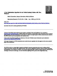
Fig 3 denotes type3 service. Each node in routing path can be divided into 3 kinds of customer sites; customer site for sending request, customer site for receiving request, and the site where there is no request any types of service. The node (1,1) becomes a base point. Fig 3-(d) describes the kinds of nodes. Fig 3-(a), for instance service type 1, shows an optimal path to collect packages into the base point from customer sites.

(5)

e ( 2, 0),(3,0 ) , e (3,0 ),(3,1) , e (3,1),( 2,1) , e ( 2,1),( 2, 2 ) , e ( 2, 2)(3, 2) , e (3, 2),(3,3) , e (3,3),( 2,3) , e ( 2,3),(1,3) , e (1,3),( 0,3) , e ( 0,3),( 0, 2) , e ( 0, 2),(1, 2) , e (1, 2 ),(1,1) } Fig 2 shows the shortest path which connects only the customer sites which request some kinds of package delivery service among the 16 customer sites. Node (1,1) is the departure of vehicle and the grayed nodes, (0,0), (1,0), (2,1), (3,2), (2,3), (1,3), are the customer sites that the vehicle have to pass by. The reason that the node (1,2) does not request any services is in the route is there is no path between node (1,3) and (1,1) so that the vehicle can reach to node (1,1) from node (1,3).

As a result of type2, fig 3-(b) shows an optimal path to deliver packages which are already collected in base. Node (1,0), (3,2), and (1,3) become via to go to other node in this route. Fig 3-(c) shows an optimal delivery route for type 3 service. A vehicle loads the packages at the base point and delivers them to the customers and collects the packages into base point from the customer sites simultaneously. In this case, the routing path may be different to the routing path which is summed with two paths of fig 3-(a) and fig 3-(b) physically. Fig 3 representing by graph notation is as follows. G(a), G(b), and G(c) are corresponded to each fig 3-(a), (b), and (c). G (a ) = (V , E ) V = { v0,0 , v0,1, v0,2 , v0,3 , v1,0 , v1,1, v1, 2 , v1,3 , v2,0 , v2,1, v2, 2 , v2,3 , v3,0 , v3,1, v3, 2 , v3,3 } E = { e(1,1),(0,0) , e(0,0),(1,0) , e(1,0),( 2,1) , e( 2,1),(3, 2) , e(3, 2),( 2,3) , e( 2,3),(1,3) , e(1,3),(1, 2) , e(1, 2),(1,1) }

Proceedings of the 7th WSEAS International Conference on Neural Networks, Cavtat, Croatia, June 12-14, 2006 (pp132-138)

G (b) = (V , E ) V = { v0,0 , v0,1, v0, 2 , v0,3 , v1,0 , v1,1, v1, 2 , v1,3 , v2,0 , v2,1, v2, 2 , v2,3 , v3,0 , v3,1, v3, 2 , v3,3 } E = { e(1,1),(0,0) , e(0,0),(1,0) , e(1,0),( 2,0) , e( 2,0),(3,1) , e(3,1),(3, 2) , e(3,2),( 2,3) , e( 2,3),(1,3) , e(1,3),(0, 2) , e(0, 2),(1,1) }

G (c) = (V , E ) V = { v0,0 , v0,1, v0, 2 , v0,3 , v1,0 , v1,1, v1,2 , v1,3 , v2,0 , v2,1, v2, 2 , v2,3 , v3,0 , v3,1, v3, 2 , v3,3} E = { e(1,1),(0,0) , e(0,0),(1,0) , e(1,0),( 2,0) , e( 2,0),( 2,1) , e( 2,1),(3,1) , e(3,1),(3, 2) , e(3, 2),( 2,3) , e( 2,3),(1,3) , e(1,3),(0, 2) , e(0, 2),(1,1) }

(a) Routing path for package gathering service.

(d) Nodes used in fig. 3 Fig.3. Results for type3 service. In type 4 service, the vehicle loads packages at the base point and delivers them to the customer sites and collects packages from customer sites simultaneously. This scenario is the same with the case of type 3 service. However, the vehicle can deliver the packages to the customer before reaching the base point if the vehicle already took the packages and does not visited the receiver’s site yet and is going to visit the site in this route. If constraints are given in Fig. 4-(a) and the optimal path is calculated according to the type 3 scenario, then the optimal path is like the result of Fig. 3-(c). In this result packages gathered at node (1,0) can be delivered to node (3,1), but packages gathered at node (2,1) cannot be delivered. So, to get optimal route for delivery, the vehicle visits node (2,1) before node (2,0). Therefore, the optimal solution for Type4 service is shown in fig. 4-(b).

(b) Routing path for package delivery service

(c) Routing path for package delivery and gathering service

(a) Constraints for package delivery

Proceedings of the 7th WSEAS International Conference on Neural Networks, Cavtat, Croatia, June 12-14, 2006 (pp132-138)

of determine the travel route of maximize the total benefit acquired by all the vehicles.

E = −∑im Benefiti + w1 * ∑im Cost i − w2 * ∑im Si S i = −(

| Li |

∑ Li | m i |

× Log

| Li |

∑im | Li |

)

(9) (10)

where m denotes the number of vehicles. Si is the entropy term to make the vehicle’s workload be distributed equally, and w is the weight factor. Li denotes the number of sites that vehicle i has visited. (b) Routing path for type4 service (a). Fig.4. Results for type 4 service.

4. Energy Function for ESA The Package delivery problem is well-known problem as extension of the TSP. The customer site with its own packages is given. A vehicle at a base point is required to visit k(≤ N) customer sites and return to the base point again. The key issue of PDP is to determine the travel route which maximizes the total number of the delivering packages and minimizes the length of the route. The benefit and the cost function for solving PDP are defined as follows: (6) Benefit = ∑ µi N i i

where, µi and N i denote the weight of the site i and the number of appearance of site with the profit µi in the travel route respectively. Cost = ∑ e (i , j ),( k ,l )

(7)

where, e(i , j ),( k ,l ) is the Euclidian distance between node (i,j) and (k,l). So, the cost function of extended simulated annealing for PDP is E = Benefit + w * Cost (8) In package delivery routing problem for multi vehicles, there are n customer sites with m vehicles. Each vehicle at a base point is required to visit k customer sites, k≤n-m+1, and return to the base point and each customer site is to be visited by the one vehicle only. A cost is incurred if a vehicle visits customer sites. Finding multi vehicle routing problem is the problem

5. ESA algorithm for PDP In ESA the states of the system build a form of Markov chain by changing the number of molecules. ESA for PDP is an open system and this fact gives rise to the following three perturbation schemes to decide a next state of the system with N molecules: (i) Increasing scheme: make a system with N+1 molecules. It is needed to select one molecule from the outside and add it to inside. (ii) Decreasing scheme: make a system with N-1 molecules. It is needed to delete one molecule from the inside. (iii) Internal swapping scheme: make a system with the same number of molecules. It is needed to interchange one molecule with another molecule in a system. (iv) External swapping scheme: make a system to have a same number of molecules by exchanging a molecule from a system with a molecule in the other system. These perturbation schemes are used in the following ESA algorithm for the PDPs. Step 1: Set initial and final temperature value. Step 2: Select one of the above perturbation schemes(i,ii,iii) randomly and perturb a current tour route s with n cities to s’ by the scheme. Perform one of the following steps(2.1,2.2) randomly. 2.1 Select two tour routes randomly, perturb a route by the perturbation scheme(ii) and the

Proceedings of the 7th WSEAS International Conference on Neural Networks, Cavtat, Croatia, June 12-14, 2006 (pp132-138)

other one by the perturbation scheme(i) to make the route s ’. It should be noted that the city to be deleted in one route must be added into the other route. 2.2 Select one system randomly and perturb a current state by the perturbation scheme(iii) to be the state s’. Step 3: Compute the benefit B(s’) which is the difference between profit and cost and compare it with the B(s) of the current state s, and let the state s’ be the new state with probability P:

P(s ' ← s) ⎧ 1 if B ( s ' ) ≥ B ( s ) (9) ⎪ =⎨ − ( B ( s ' ) − B( s )) ) if B ( s ' ) 〈 B( s ) ⎪exp( kT ⎩ Step 4: Repeat step 2 and 3 until the equilibrium state occurs. Step 5: Anneal with an annealing schedule. Step 6: Repeat step 2, 3, 4, and 5 until reaching to the final temperature.

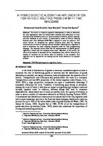
Fig. 5. Final route for type3 service.

7. Conclusion 500.0

Energy Tourlength Weight

450.0 400.0 350.0 300.0

6 Experimental and Results Fig 5 shows the data and the final routing path for type 3 service. 7*7 mesh nodes are used for experiment. The gray-scaled node means sender site and the thick circle means the receiver site. The gray-scaled thick circle represents sender and receiver site at the same time. Node(3,3) is the base point. Fig 6 and 7 show the result of 2 vehicles PDP with 49 customer sites. In Fig 5 node(3,6) is included into the path even though it is not a sender site as well as a receiver site. The node(3,6) plays a role of the bridge between node(4,6) and node(2,6). Fig 6 shows the energy, distance, and weight values from the initial state to the final state for the routing path shown in fig 5. Fig 7 shows the number of sites that the vehicle visited.

250.0 200.0 150.0 100.0 50.0 0.0 1

51

101

151

201

251

Fig. 6. Progress of the convergence. 45

Truck1 Truck2

40 35 30 25 20 15 10 5 0 1

51

101

151

201

251

Fig. 7. the number of customer sites that vehicles visited.

Proceedings of the 7th WSEAS International Conference on Neural Networks, Cavtat, Croatia, June 12-14, 2006 (pp132-138)

In this paper, we define a new concept of multi Package Delivery Problem and show how can be solved the PDP in real world applications applying ESA. The mPDP can be considered an extension of multi salesmen problem. We define 4 services of package delivery and show the optimum routing path for each service. In energy function for ESA benefit and cost are used, which mean the number of appearance of site with the profit and the Euclidian distance between nodes. Experimental results show the optimal routing path for 49 customer sites. The described Package Delivery Problem can be extended to the problem which minimizes the delivery distance and maximizes the weight(or value) of the package at the same time. The proposed algorithm can be applied to the problem that finds the shortest path to collect and deliver packages at the same time. Reference : [1] Wee-Kit Ho, Andrew Lim and Wee-Chong Oon, ‘Maximizing Paper Spread Examination Timetabling Using a Vehicle Routing Methos’, Tools with Artificial Intelligence, Proceedings of the 13th International Conference on, [2] Chi-Hwa, S., KyungHee, L and Wondon, L. ‘Extended Simulated Annealing for Augmented TSP and Multisalesmen TSP’, IJCNN 2003 Portland Oregon July 20-24, 2003. [3] Guoxing, Y. ‘Transformation of multidepot multisalesmen problem to the standard traveling salesman problem’, European Journal of Operational Research 81, 1995, pp 557-560. [4] Kirkpatric, S., and Gelatt, C., and Vecch, M. ‘Optimization by simulated annealing’, Science, 1983, 220 pp. 671-680.