Genetic Algorithm Based Approach for Designing Computer Network ...

Genetic Algorithm Based Approach for Designing Computer Network Topologyt Anup Kumar*, Rakesh M. Pathak’, M. C. Gupta’

lEngrg.

Math. and Computer Science ‘bepartment of Management University of Louisville Louisville, KY 40292

Yash P. Gupta Office of Dean College of Business University of Colorado Denver, CO 80202

reliability,

Abstmct: Gne of the important features of computer networks is the potential for high reliability. The reliability of a network depends on many parameters such as connectivity, degree of each node, and average distance between any pair of nodes. The main focus of the problem considered in this paper is to design reliable computer network topologies. A generalized framework based on Genetic Algorithm is developed which is applicable to wide range of network design problems. Several topology design problems are solved to demonstrate the generality of this solution approach. The results obtained from genetic algorithm based solution approach are compared with the optimal solutions to illustrate the effectiveness of the proposed approach.

I.

Introduction

The advent of low cost computing devices has led to the explosive growth in the area of computer networks. There are several benefits to be achieved by this dispersal of computing across a network such as resource sharing and improved reliability. Che of the major advantages of computer networks over the centralized systems is their potential for improved system reliability. The reliability of a system dependsnot only on the reliability of its nodes and communication links, but also on the fact how nodes are connected by communication links. A completely c-o~ected network has the highest computer network reliability [l] whiiethe simple loop network has the lowest computer network reliability. In order to design a network with high

The topology of a network can be represented by a linear graph. These network topologies can be characterized by their network reliability, messagedelay or the capacity of the network. These performance characteristics of a network depend on many properties of linear graphs which represents the network topology [2-51. These properties are diameter, average distance, number of ports at each node, and number of links in a network. The definition of these properties is provided in section 2.3. Diameter has the direct relationship with the delay in the network [S]. Higher the diameter, larger the delay in the network. Diameter, average distance and number of links have direct impact on the system reliability [3,5]. Reliability increases with the decreasein diameter and average distance, while a decrease in number of link reduces the system reliability. The key to network design is to formulate the problem in terms of cost factors and constraints. The objective here is to design a network such that the cost factor(s) (represented by a cost function) are optimized and all the constraints are satisfied. The nature of a cost function and the constraints depend on the type of problem at hand. For example, response time in real time systems is extremely critical, while in communication%wetworks other parameters such as throughput or system reliability may be more important. Performance oriented cost functions have dominated the literature [2-81 for network design but there arc very few algorithms optimizing the reliability of a network. The algorithms proposed Hakimi, Pradhan, Aggrawal, Wilkov [g-12] provide a good starting point for designing reliable network topologies. The existing schemesdo not optimize the overall reliability [ 131but try to improve the reliability bounds only. In most of the design problems the reliability and the availability parameters are used as constraints but not as the objective functions. The scheme proposed in [2]

‘This research is in part supported by Telecommunications Research Center.

Permission to copy without fee all or part of this material is granted provided that the copies are not made or distributed for direct commercial advantage, the ACM copyright notice and the title of the publication and its date appear, and notice is given that copying is by permission of the Association for Computing Machinery. To copy otherwise, or to republish, requires a fee and/or specific permission.

0 1993 ACM O-89791 -558-5/93/0200/0358

the topology should be as close to fully as Possible. But it is not plausible to design a highly reliable system as completely connected network [l] due to high cost of construction. co~ected

$1.50 358

is very complex and does not optimize the exact reliability. In addition, the existing schemes are not suitable for designing non regular network topologies (topologies where nodes may have different connectivity pattern). Most of the complex distributed network topologies are not regular. This paper addressesa general&d framework for designing any type of topology.

2.3 Definitions: Diameter: Diameter of a network is defined as the maximum of minimum distances between any pair of nodes. It can be represented as follows: = 1, diameter = max {DU: foralli = 1,2, ..,N,andallj 2 , ..,N) Average Distance: It is defined as follows:

In this paper, we have addressed various types of problems for network design. These problems deal with optimization of diameter, average distance, and computer network reliability. An extended framework is developed that can solve all these problem with minor modifications.

N c i=l Al)

N C Drj j=l

=N(N-1)/2

The rest of the paper is organized as follows. Section II defines the network design problem. Background of Genetic Algorithms is discussed in section III. An algorithm for solving the network design problem is discussed in section IV. Section V provides the results of various problems specified in section II. Concluding remarks are included in section VI. II.

Degree: Degree of a node is defined as the number of links incident to the node. Computer Network Reliability (CNR): It is defined as the probability of each node communicating with all the other nodes in a given network [ 141. In order to compute the CNR, first all the spanning trees of the networks are computed then these trees are made disjoint using the algorithm [ 141.

Problem Development

In this section, we first specify various terms and notation used in explaining the concepts outlined in subsequent sections. There after, we introduce the definition of various parameters used in the paper and then list assumptionsmade in representing the network topology.

In this paper several network design problems have been solved for optimizing the computer network reliability, diameter and average distance. Mathematically, these problems can be defined as follows:

2.1 Notation N: Total number of nodes in the computer network g : Total number of strings in a generation G(i):Represents the i* generation Do: Minimum number of hops between nodes (i) and (i). deg$Degree of a node (i). 1; if there is a communication link between nodes(i) and (j) 4 = 0; otherwise Of;: Fitness value of string number i in a generation Suq:Sum of the fitness values of all the strings in generation number j 2.2

Assumptions

i. A network topology is modeled by a graph G, where nodes represent the processing elements, and edges denote the communication links. ii. A graph G does not have any self loops. iii. Failure of a link is independent of failures of other links. iv. A link has only two states: operational or faulty.

359

Problem 1: CNR Under Diameter Constraint Given: Number of nodes, link reliability values, desired diameter of the network @) Objective Function: Maximize computer network reliability Constraint: Max [Dii: for all i = l,..N; andallj = l,.., N] = D Problem 2: Diameter Under Degree Constraint Given: Number of nodes, upper botqd on degree of each node (deg,) Objective function: minimize diameter Min {Max [Dij: for all i = l,..N; and all j = l,..,N’l} Constraints: M c Lij s degj ; for each node (i) 15j zzN f-1 Problem 3: Average Distance Under Degree Constraint Given: Number of each node, upper bound on degree of each node (deg,) Objective function: minimize average distance N N c C D, i=l j=l ------------AD= N(N-1) / 2

. randomly select two chromosomes . shuffle them to generatenew offsprings . compute the fitness value of new offsprings } add these offsprings to G(i + 1) \ Until (enough offsprings are in generation G(i + 1)

Constraints:

$ L,j i-1 III

4 degl ; for each node (i) 1 s;jsN

Generalized Solution Approach

-i = i+l} Until (Termination Condition is Satisfied)

The generalized solution methodology based on Genetic Algorithm is proposed for network design. Genetic Algorithm (GA) [ 151was developed by John Holland at the University of Michigan. Genetic algorithms are search techniques for global optimization in a complex search space. As the name suggests, GA employ the concepts of natural selection and genetics. Using past information GA direct the searchwith expected improved performance. The concept of genetic algorithm is based on the theory of adaption in natural and artificial systems [15]. In artificial adaptive systems, adaptation starts with a initial set of structures (possible solutions). This initial structures are modified according to the performance of their solution using an adaptive plan [15] to improve the performance of these structures. It is proved by Holland that repeatedly applying this adaptive plan to input structures results in optimal or near optimal solutions [15]. The traditional methods of optimivltion and search do not fare well over a broad spectrum of problem domains [16]. Some are limited in their scope because they employ local search techniques (e.g. calculus based methods). Others, such as enumerative schemes, are not efficient when the practical search space is too large.

There are three main steps in the repeat loop for GA: 1. The process of selecting good strings from the current generation to be carried to the next generation. This process is called reproduction / selection. 2. The process of shuffling two randomly selected strings to generate new offsprings is called crossover. Some times one or more bits of a chromosome are complemented to generate a new offspring. This process of complementation is called mutation. 3. Computation of fitness value using objective function. The population size is finite in each generation of GA, which implies that only relatively fit chromosomes in generation (i) will be carried to the next generation (i + 1). The power of GA comes from the fact that, the algorithm terminates rapidly to an optimal solution. The iterative process terminates when the solution reaches the optimum value [16]. The three genetic operators namely selection, crossover and mutation are discussed next in detail: 3.2 Selection / Reproduction: Since population size in each generation is limited, only finite number of good chromosomes will be copied in mating pool depending on the fitness value. Chromosomes with higher fitness values contribute more copies to the mating pool than those with lower fitness values. This can be achieved by assigning proportionately a higher probability of getting copied to a chromosome with higher fitness value [16,17]. Selection / reproduction uses the fitness values of the chromosome obtained after evaluating the objective function. It uses a biased roulette wheel [14] for selection of chromosomesto be taken in the mating pool. It ensures that highly fit chromosomes (with high fitness value) have a higher number of offsprings in the mating pool. Each chromosome (i) in the current generation is allotted a roulette wheel slot sized in proportion (pi) to its fitness value. This proportion pi can be defined as follows. Let

3.1 Concept of Genetic algorithm In GA, search spaceis composedof possible solutions to the problem. A solution in the search space is represented by sequenceof O’s and 1’s. This solution string is referred as the chromosome in the search space. Each chromosome has associatedobjective function value called jitness value. A good chromosome is the one that has high/low fitness value depending upon the problem The strength of a (maximization/minimization). chromosome is represented by its fitness value. Fitness value indicates which chromosome are to be carried to the next generation. A set of chromosomes and associated fitness values is called the population. This population at a given stage of GA is referred to as a generation. The general GA proceeds as follows: Start with initial set of chromosomes in generation G(0) Set i = 0 repeat { - Select good chromosome from G(i) to be carried to G(i + 1) - repeat { . From the pool of selected chromosomes {

ofi = the actual fitness value of a chromosome (i) in generation (i) of (g) chromosomes Q sumj = c Of i ; total Of the fitlESs values Of all i=l chromosome8 in generation j.

360

pi = Of,/SUmj

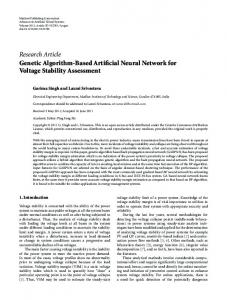
Number of copies of chromosome (i) in the mating pool = N Pi When roulette wheel is spun, there is greater chance that better chromosome will be copied into the mating pool because a good chromosome occupies large area on the roulette wheel. 3.3 Crossover: This phase involves two steps: first, from the mating pool, two chromosomesare selected at random for mating, and second, a crossover site c is selected uniformly at random in the interval [ 1, N-l]. Two new chromosomes, called offsprings, are then obtained by swapping all characters between positions c and N. This can be shown using two chromosomes, say A and B, each of length 6 bit positions:

A: B:

10 111 0 1010

node network can be represented as follows: N* NI N3 --Y-s---% Nz N, N,, No Nx, &, Nn Nss ---------1-P--In this representation, there are three node fields for Nl , N2, N3. Each of these node fields has three bits becausethere are three nodes in the network. These bits N, indicate whether there is a connection between node Ni and node Nj. In a chromosome, each Nij, (1 < iJ 4 3), is represented by 0 or 1 according to the following convention: 1; if node Ni is COMeCted to Nj N, = 0; Otherwise An example shown below will illustrate the organization and meaning of a chromosome used in solving network design problem.

0 1 11

Let crossover site c be 3. Then the two offsprings can be obtained as follows: contribution from A contribution from B c: 101 011 contribution from B contribution from A D: 010 101 This ensures that each new offspring gets a complete chromosome containing all the constituent information about the coded parameter (since each bit position represents some unique characteristic). 3.4 Mutation: The combined operation of reproduction and crossover may sometimes lose some potentially useful information from chromosome. To overcome this problem, mutation is introduced. It is implemented by complementing a bit (0 to 1 and vice versa) at random. This ensures that good chromosomes are not permanently lost. IV. Genetic Algorithm and Network Design Problem In this section, we discuss the details of GA developed for solving the network design problem. The development of GA requires i) Chromosomal coding scheme, ii) Initialization, iii) Genetic crossover operator, iv) Network operator, v) Replacement strategy and vi) Termination rules.

N2 101

N3 110

Nl 011

This chromosome indicates that: (1) node 3 is co~ected to nodes 1 and 2, (2) node 2 is co~ected to nodes 1 and 3, and (3) node 1 is connected to nodes 2 and 3. In general, if there are N nodes in the network then chromosome will be represented as follows: N ~“........~... N, N* ----_-------------___I__ N,,&,..%, WwNm..Nm ....... %Nz,..Nm ------------------------------4.2 Genetic Crossover Operators: The genetic crossover operators used in the development of this algorithm is called Random Node Field Swap wtor (RNFSO). In RNFSO, one of the node fields is swapped randomly at a time in the chromosome. User can specify the total number of node fields to be swapped for the crossover. Random numbers are generated (0, N-l) for swapping specified number of node fields. For example string 1 string 2

110 010

101 101

011 010

If only one node field is to be swapped then a random number is generated to decide which field to be swapped. Let the field to be swapped is 3, then RNFSO wilI provide the following results: Child 1 010 101 011 Child 2 110 101 010

4.1 Chromosomal Coding: Since our problem involves the representation of connection between nodes, we have employed a coding scheme using binary numbers. The complete chromosome of network connectivity is divided in node fields which are equal to number of nodes in the network. One arrangement of connection between three

361

The crossover operator sometimesgeneratesa chromosome which does not represent a proper network. For example in child 2, node field N3 indicates that N3 is connected to nodes Nl and N2 but node field Nl indicates that Nl is connected to only node N2. This anomaly is corrected by network operator discussed in section 4.3. 4.3 Network Operator: Since these crossover operators produce discrepancy in the chromosome a simple procedure called “network operator” is executed as follows:

4.5 Genetic Algorithm Parameter There are four parameter that affect the solution obtained from GA based GRIP. These parameters are crossover rate (PCRS), mutation rate (PMRS), population size (PPSZ) and number of generations (PNOG). The detailed analysis and experiments for choosing the appropriate parameter values is considered by De Jong and Grefenstette in [18]. These parametric studies suggest that good GA performance requires high PCRS, very low PMRs and moderate PPSZ. Based on these observations Goldberg [ 16,181 indicates that the appropriate value of PCRS is 0.6 and PMRS is .033 and PPSZ is about 30. The affect of PPSZ and PNOG on the value of objective function obtained from GRIP is discussed in section V.

Network Operator: for each swapped node field (N,) in a chromosome forj = l,N If bit Nrj = 1 then If Nj,, = OthenNj,,= 1; else If bit Nj., = 1 then Nj,t = 0; end for; end for; It can be illustrated with the example from SNFSO, where child 1 and child 2 do not represent a valid topologies. For child 1 Node field N3 is modified after crossover. Thus for swapped node field N3, bit NJ2 is 1 and bits N,, , Nsa are 0. This implies bit Nrr should be 1, W3 =0, N, = 0. The valid chromosome after performing adjustment is: Child 1

010

101

crossover is added to the new generation if it has a better objective function value than both of its parents. If the objective function value of an offspring is better than only one of the parents, then we select a chromosome randomly from better parent and the offspring. If the offspring is worst than both parent than any one of the parent is selected at random for the next generation. This ensures that the best chromosome is carried to the next generation, while the worst is not carried to the succeedinggenerations.

4.6 Termination Rule The execution of the GA based GRIP can be terminated when the number of generations exceed an upper bound specified by the user. The upper bound on the number of iterations in GA must be specified carefully [16,17] to ensure that best objective function value is obtained with in the iterations specified.

010

This network operator preserves the crossover characteristics by adjusting the chromosomes according to newly acquired node fields. The impact of the network operator is same as mutation process since it randomly selects a bit position in chromosome and modifies it to its complement.

4.7 Algorithm Development The genetic algorithm starts with an initial generation of valid chromosomes which satisfy the constraints of the problem type. The initial generation contains a finite number of valid strings selected at random. The number of strings in any generation, called the population size, is kept even to ease the process of crossover.

4.4 Replacement Strategy This subsection discussesa method used for creating new generation after crossover, mutation and adjustment is carried out on the chromosomes of previous generation. There are several replacement strategies exist in the literature, a good discussion can be found in [ 181. The most common strategy is to probabilistically replace the poorest performing chromosome in the previous generation. The elitist strategy appends the best performing chromosome of previous generation to the current population and, thereby, ensures that the chromosome with the best objective function value always survives to the next generation.

Algorithm for Network Design: Step 1: (Initialization) Initialize PCRS, PMRS, PPSZ and PNGG. i = 0. Read the distributed system parameters such as number of nodes, degree of node, link reliability, diameter and average distance, value of g, etc. Generate initial population G(i) randomly of size g. Step 2: (Fitness Value) Compute CNR for eachchromosome in the generation G(i) for Problem 1. Compute the diameter in generation G(i) for problem

The algorithm developed here combines both the above mentioned concepts. Each offspring generated after

362

-

2. Compute the average distance in generation G(i) for problem 3.

Step 3: (Reproduction / Selection)

Perform selection on G(i) to form the mating pool as discussed in section 3.2 Step 4: (Shuflling): Apply SNFSO or RNFSO to chromosomes in the

-

mating pool with probability PCRS. Apply mutation with probability PMRS. Apply network operator to new offsprings. Check for constraints: If the constraints are not satisfied discard the chromosomesand go to step 4.

Step 5: (Replacement and creation of new generation) If number of chromosomes in generation G(i + 1) > g then go to Step 6. m Apply replacementstrategy discussedin section 4.4 to add chromosomes in generation G(i). Go to step 4. Step 6: (Terminating Conditions) i=i+l If the terminating condition is not satisfied then go to step 2 else STOP. V.

Numerical

Examples

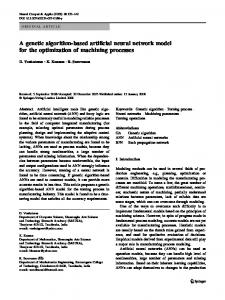
This section provides the detailed results obtained for the three problems discussed in section II. For each of the three problems several network topologies are designed using GA based approach. The objective function values obtained from the GA approach are compared with the optimal results computed using exhaustive search of complete solution space.Impact of number of generation on the optimal objective function value is also discussed for each of the three problems. Initial population in each case was chosen randomly. The algorithm terminates using the criteria given in section 4.6. 5.1 CNR Under Diameter Constraint Problem: In this problem a network is to be designed such that computer network reliability is maximized and the requirement for specified diameter must be met. Several networks are designed for various node numbers. The problem is solved for four different caseswhen the number of nodes in the network are 6, 7, 8, and 9. The constraint for diameter for various networks of different nodes is shown in Table I.

The topology resulted from GA for 6 node network with diameter constraint of 2 is shown in Table II. Each row in the table represents one topology for a given problem size. The first column in the Table II indicates the number of nodes in the network. Remaining columns provide the connectivity information of the network. The first row of Table II describes the network topology of 6 nodes, where column for Nl indicates that node 1 is to connected to nodes 2, 5, and 6; node N2 is c~~&ed nodes 1, 3, and 4. Similarly other fields can be interpreted for their connection. The overall CNR for the topology generated for 6 node network is .9932. The CNR of topologies obtained from GA for networks with 6, 7, 8, and 9 nodes are compared with optimal solution to establish the accuracy and validity of genetic algorithm approach. The optimal solutions for these problems were obtained using exhaustive search of complete solution space. The CNR of topologies obtained from GA and the optimal CNR computed using exhaustive search is given in Table III. It is clear that GA algorithm generates topologies that have optimal CNR.

1

I

OS932

6

I

I 0.9597

7

0.9470

0.0

I 0.9597

I

I

8

I

0.9932

0.0 1

0.9470

0.0

5.2 Minimum Diameter Under Degree Constraint:

5.3 Average Distance Under Degree Constraint:

In this problem a network is to be designed such that the diameter of the network is minimized and the degree of each node is less than or equal to the specified value. The problem is solved for four different caseswhen the network has 6, 7, 8, and 9 nodes. The upper bound on the degree of each node in these casesis specified in Table IV.

In this problem a network topology is to be designed such that the average distance is minimized and degree of each node must satisfy the specified constraint. The problem is solved for networks of sixes 6, 7, 8, and 9 nodes with the upper bound on the degree of each node is specified as shown in Table IV.

lwelvtDcgrccofacb

Mdc

In order to validate the optimality of these solutions, the average distance of the topologies obtained for networks from GA are compared with optimal values computed from exhaustive search. The results are reported in Table VII.

Nodes

The diameters of the topologies generated by GA is compared by optimal solution obtained by exhaustive search. The results for networks having 6, 7, 8, and 9 nodes are reported in Table V. As we can observe in all the casesGA provides optimal solution. The connectivity of the optimal network topologies obtained using GA are given in Table VI. Each row in the table represents the network topology. The first column shows the number of nodes in the network. The remaining columns provide the connectivity of the network. This connectivity can be interpreted as discussed in section 5.1.

Node

Diameter(GA)

Diicu(Op)

+Diff

6

2

2

0

7

2

2

0

NI

N2

N3

I

N4

NS

1

I

L3.4.6 4.6.78

I

l.Z3,6

L&247

3,Y*7

1,47,8

Z4AfJ

(GA)

COP)

96 DEL

6

1.u)

1.20

0.0

7

1.33

1.33

0.0

8

1.42

1.42

0.0

9

150

1.50

0.0

In all the three problem we have shown the comparison of optimal solution for networks having 6, 7, 8, and 9 nodes because it is extremely computation intensive to evaluate the optimal solution for larger networks. To get an idea of the computation time requirement for performing exhaustive search, consider the 9 node network example. Computing the optimal solution for the 9 node network using an exhaustive required approximately 18 hours of computing time. This time increases exponentially with the increase in the number of nodes in the network.

6

8

Av. Dis

The GA algorithm provided the optimal solution in every case for this problem. The connectivity of the optimal topologies for various csses of this problem is shown in Table VIII. Each row in the table represents the network topology. The first column gives the number of nodes in the network. The remaining columns provide the connectivity of the network. This connectivity can be interpreted as discussed in section 5.1.

N9

N6

Av. Dir

3J.W VA8

+

364

[7] o&s

Nl

N2

N3

N4

NS

N6

Nl

N8

N9

6

2A4.6

1.3.4.5

1,2$,6

lJ.5.6

2A4.6

1.3.4.5

-

-

-

[S] [9]

7

1 24J.6 1 1,3,4,7 1 2,.5,6,7 ) 1J,5,6 1 LX4.7 1 lA4s7 1 ZU6

1

-

1

-

8

24S.6

1,3,7,8 fU.8

L3.6.8

1,3&S

1,4..5,7 Y,68

U.4.7

9

24.6.9

1.479

I#.1

3.4.8.9

1.2.3.8 2A4.8

5.6.7.9 QA8

4,5,6,7

1

[lo]

-

[ll] VI. Conclusions In this paper a generalized schemebased on Genetic Algorithms is developed to solve network topology design problem. This schemeis applicable to any type of network design problem. This is demonstratedby solving the same problem using three different objective functions. This algorithm can also design topologies for performance oriented network parameterssuch as throughput and delay. The validity of this approach is established by comparing results from GA with the optimal solutions obtained by exhaustive search of complete solution space. It is also possible to use multiple objective functions for designing the networks. Currently, we are extending this work for multiple objective functions.

[l2]

[13] [14]

[15]

Regarding future research issues GA based approach can be applied to many distributed network design applications such as file allocation problem, reliability improvement of distributedsystems and network expansion.

[16] [17]

References

Dl D. P. Agrawal, ” Advanced Computer Architecture (Tutorial)“, IEEE Computer Society Press, June 1986, 383 pages. K. B. Irani and N. G. Khabbaz,“A Methodology for PI the Design of Communication Networks and the Distribution of Data in Distributed Supercomputer Systems”, Vol. C-31, No.& 1982, pp. 419-434. r31 L. Kleinrock,“Analytic and Simulation Methods in Computer Network Design”, Proceedings of Spring Joint Computer Conference, 1970, pp. 569-579. r41 H. Frank and W. Chou, “Topological Optimization of Computer Networks ” , Proceedings of the IEEE, Vo1.60, No.11, 1972, pp. 13851397. PI R. S. Wilkov,“Analysis and Design of Reliable Computer Networks, “IEEE Transactions on Communications, pp. 660-678, 1972. El R.R. Boorstyn and H. Frank, “Large Scale Network Topological Optimization,” IEEE Trans. Communications, COM-26, Jan. 1977, 29.47.

[U]

365

S.P. Jain and K. Gopal, “On Network Augmentation, ” IEEE Trans, Reliability, R-35, Dec. 1986, 541-543. H. Frank and R.E. Kahn,“Computer Communication Network Design, ” AFIPS-Conference Proceedings, vo140, pp. 255-313. S.L. Hakimi, A.T. Amin, “On the design of reliable networks”, Networks, ~013, 1973, pp 241-260. D. K. Pradhan and S. M. Reddy,“A Fault tolerant communication architecture for distributed systems,” IEEE Transactions on Computers, Vol. C-3 1, Sept 1982. K.K. Aggarwal, Y.C. Chopra and J.S. Bajwa, “Topological Layout of Links for Optimizing The Overall Reliability in a Computer Communication System,” Microelectronics and Reliability, Vol. 22, No. 3, 1982, pp. 347-351. R.S. Wilkov, Design of computer networks basedon a new reliability measure, Proc. Symp. Computer Comm. Networks and Teletraffic, pp. 371-384 (New York, April, 1972). A.Kumar, “On Evaluationof Reliability and Integrated Performance-Reliability Parameters” Ph.D Dissertation, N.C.S.U, Aug. 1989. K. K. Aggarwal and S. Rai, “Reliability Evaluation in Computer Communication Networks”, IEEE Transactions on Reliability, Vol. R-30, June 1981, pp. 32-35. J. H. Holland, “Genetic Algorithm and the Optimal Allocation of Trials”, SIAM Journal of Computing, Vol. 2(2), 1973a, pp. 88-105. D. E. Goldberg, “Genetic Algorithms in Search, Optimization and Machine Learning”, AddisonWesley Publishing Company, 1989, pages412. R. M Pathak, A. Kumar and Y. P. Gupta, “Reliability Oriented Allocation of files on Distributed Systems”, Proceedings of IEEE Symposium on Parallel and Distributed Systems, pp. 886-893, Dec., 1990. K. A. De Jong,“An Analysis of the Behavior of a Class of Genetic Adaptive Systems,” Ph.D. Thesis, University of Michigan, (University Microfilm No 769381).